In the article (Warton et al. 2015) the fitting of joint species distributions models is performed using the package boral which runs with JAGS (Just Another Gibbs Sampler) a simulation program from hierarchical Bayesian models using MCMC methods implemented in C++.
This package and the package jSDM allow to fit the models defined below, so we can compare the results obtained by each of them on different data-sets.
1 Models definition
1.1 Binomial models for presence-absence data
We consider a latent variable model (LVM) to account for species co-occurrence (Warton et al. 2015) on all sites .
\[y_{ij} \sim \mathcal{B}iniomial(t_i, \theta_{ij})\]
\[ \mathrm{g}(\theta_{ij}) = \alpha_i + X_i\beta_j + W_i\lambda_j \] - \(\theta_{ij}\): occurrence probability of the species \(j\) on site \(i\). - \(t_i\): number of visits at site \(i\) - \(\mathrm{g}(\cdot)\): Link function (eg. logit or probit).
The inference method is able to handle only one visit by site with a probit link function so \(\forall i, \ t_i=1\) and \[y_{ij} \sim \mathcal{B}ernoulli(\theta_{ij})\].
\(\alpha_i\): Random effect of site \(i\) such as \(\alpha_i \sim \mathcal{N}(0, V_{\alpha})\), corresponds to a mean suitability for site \(i\). We assumed that \(V_{\alpha} \sim \mathcal{IG}(\text{shape}=0.1, \text{rate}=0.1)\) as prior distribution in
jSDMpackage and that \(V_{\alpha} \sim \mathcal{U}(0,30)\) inboralpackage.\(X_i\): Vector of explanatory variables for site \(i\) with \(X_i=(x_i^1,\ldots,x_i^p)\in \mathbb{R}^p\) where \(p\) is the number of bio-climatic variables considered (including intercept \(\forall i, x_i^1=1\)).
\(\beta_j\): Effects of the explanatory variables on the probability of presence of species \(j\) including species intercept (\(\beta_{0j}\)). We use a prior distribution \(\beta_j \sim \mathcal{N}_p(0,\Sigma_{\beta})\) with \(\Sigma_{\beta}\) a diagonal matrix of size \(p \times p\) whose values on the diagonal are fixed at \(10\).
\(W_i\): Vector of random latent variables for site \(i\). \(W_i \sim N(0, 1)\). The number of latent variables \(q\) must be fixed by the user (default to \(q=2\)).
\(\lambda_j\): Effects of the latent variables on the probability of presence of species \(j\) also known as “factor loadings” (Warton et al. 2015). We use the following prior distribution in both packages to constraint values to \(0\) on upper diagonal and to strictly positive values on diagonal, for \(j=1,\ldots,J\) and \(l=1,\ldots,q\) : \[\lambda_{jl} \sim \begin{cases} \mathcal{N}(0,10) & \text{if } l < j \\ \mathcal{N}(0,10) \text{ left truncated by } 0 & \text{if } l=j \\ P \text{ such as } \mathbb{P}(\lambda_{jl} = 0)=1 & \text{if } l>j \end{cases}\].
This model is equivalent to a multivariate GLMM \(\mathrm{g}(\theta_{ij}) =\alpha_i + X_i.\beta_j + u_{ij}\), where \(u_{ij} \sim \mathcal{N}(0, \Sigma)\) with the constraint that the variance-covariance matrix \(\Sigma = \Lambda \Lambda^{\prime}\), where \(\Lambda\) is the full matrix of factor loadings, with the \(\lambda_j\) as its columns.
1.2 Poisson model for abundance data
Referring to the models used in the articles (Hui 2016), we define the following model to account for species abundances on all sites.
\[y_{ij} \sim \mathcal{P}oisson(\theta_{ij})\].
\[ \mathrm{log}(\theta_{ij}) =\alpha_i + \beta_{0j} + X_i\beta_j + W_i\lambda_j \]
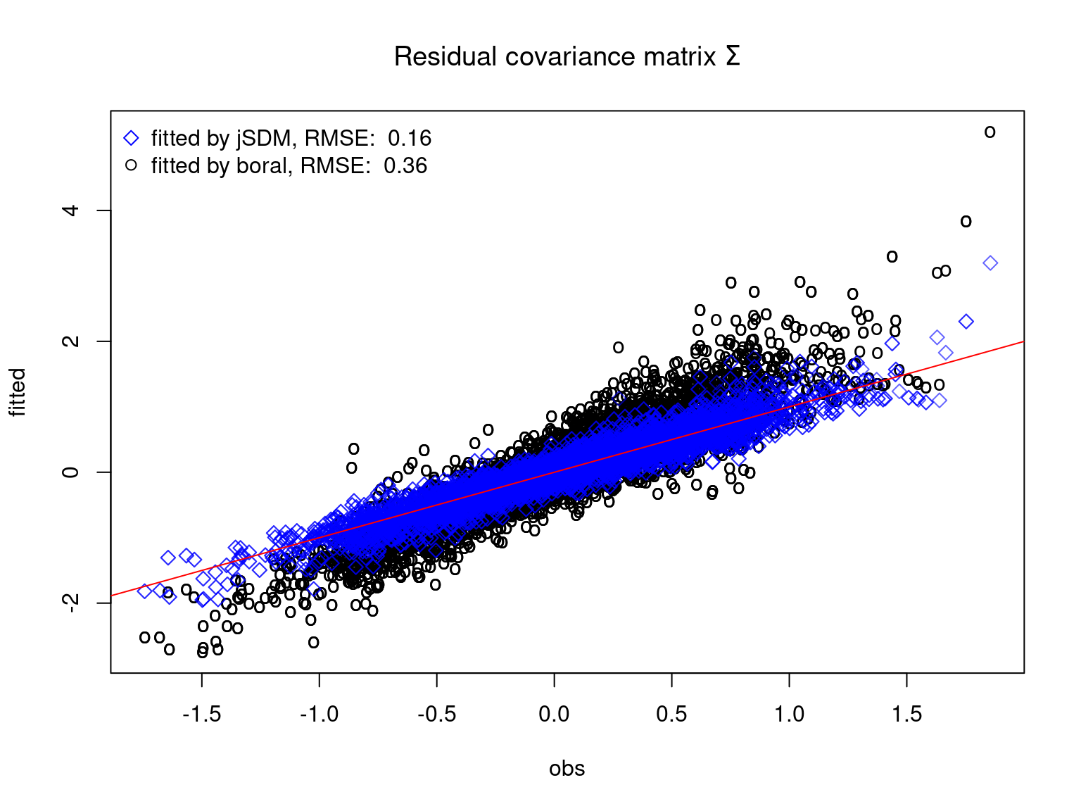
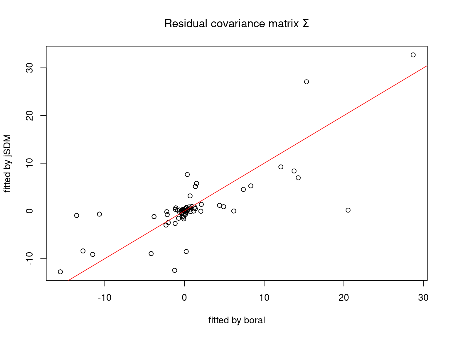
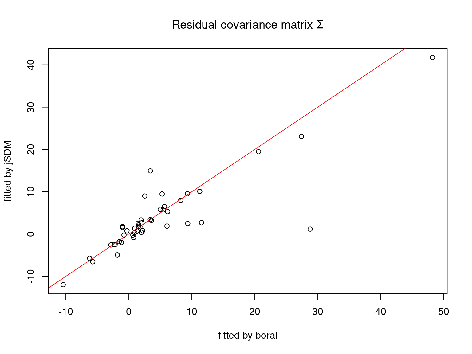
Using this models we can compute the full species residual correlation matrix \(R=(R_{ij})^{i=1,\ldots, nsp}_{j=1,\ldots, nsp}\) from the covariance in the latent variables such as : \[\Sigma_{ij} = \lambda_i^T .\lambda_j \], then we compute correlations from covariances : \[R_{i,j} = \frac{\Sigma_{ij}}{\sqrt{\Sigma _{ii}\Sigma _{jj}}}\].
2 Data-sets
2.1 Data simulation
We start by simulating the data-set that we will then analyze among real data-sets.
We generate a data-set following the previous model with \(300\) sites, \(100\) species and as parameters :
#==================
#== Data simulation
#==================
#= Number of species
nsp <- 100
#= Number of sites
nsite <- 300
#= Number of latent variables
nl <- 2
#= Set seed for repeatability
seed <- 1234
set.seed(seed)

# Ecological process (suitability)
x1 <- rnorm(nsite,0,1)
x2 <- rnorm(nsite,0,1)
X <- cbind(rep(1,nsite),x1,x2)
np <- ncol(X)
#= Latent variables W
W <- matrix(rnorm(nsite*nl,0,1), nrow=nsite, ncol=nl)
#= Fixed species effect beta
beta.target <- t(matrix(runif(nsp*np,-1,1), byrow=TRUE, nrow=nsp))
#= Factor loading lambda
mat <- t(matrix(runif(nsp*nl,-1,1), byrow=TRUE, nrow=nsp))
diag(mat) <- runif(nl,0,1)
lambda.target <- matrix(0,nl,nsp)
lambda.target[upper.tri(mat,diag=TRUE)] <- mat[upper.tri(mat, diag=TRUE)]
#= Variance of random site effect
V_alpha.target <- 0.5
#= Random site effect alpha
alpha.target <- rnorm(nsite,0,sqrt(V_alpha.target))

# Simulation of response data with probit link
probit_theta <- X %*% beta.target + W %*% lambda.target + alpha.target
theta <- pnorm(probit_theta)
e <- matrix(rnorm(nsp*nsite,0,1),nsite,nsp)
# Latent variable Z
Z_true <- probit_theta + e
# Presence-absence matrix Y
Y <- matrix (NA, nsite,nsp)
for (i in 1:nsite){
  for (j in 1:nsp){
    if ( Z_true[i,j] > 0) {Y[i,j] <- 1}
    else {Y[i,j] <- 0}
  }
}
2.2 Data-sets description
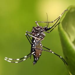
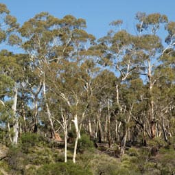
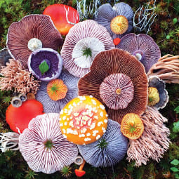
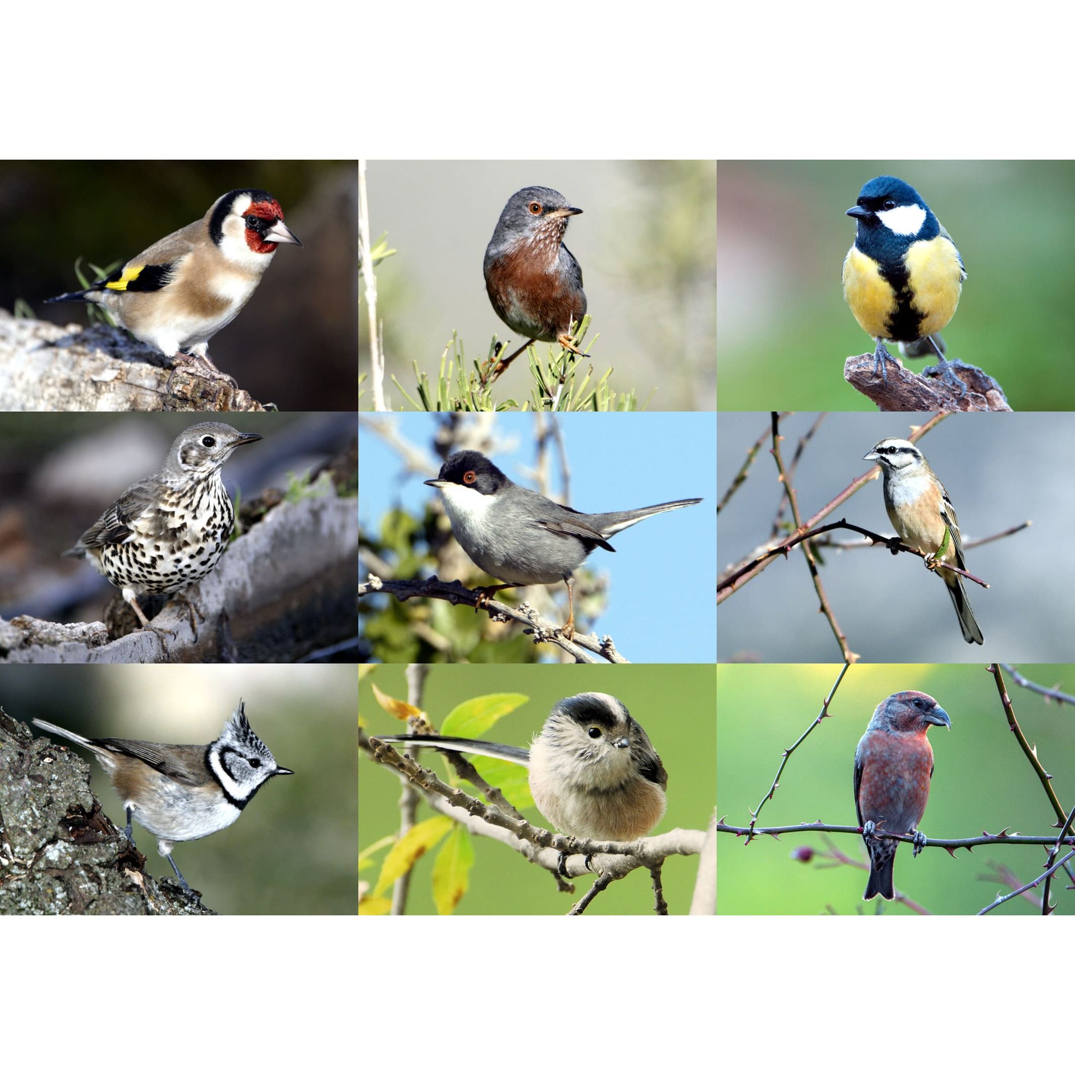
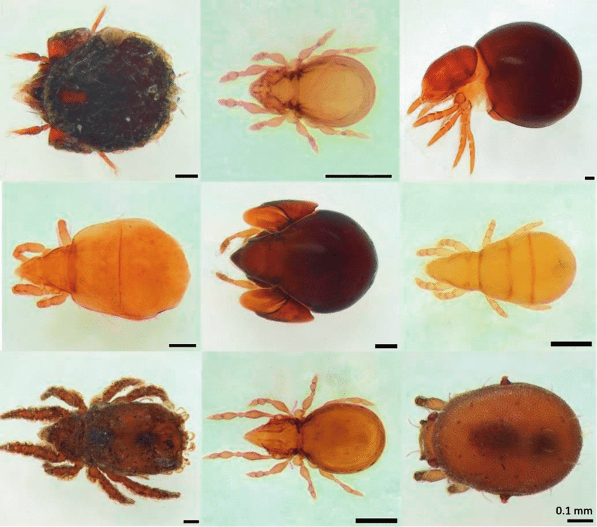
Among the following data-sets, the presence-absence data are from the (Wilkinson et al. 2019) article in which they are used to compare joint species distribution models for presence-absence data, the data-set that records the presence or absence of birds during several visits to each site is from the (Kéry & Schmid 2006) article and the mites abundance data-set is from the (Borcard & Legendre 1994) article.
#> ##
#> ## jSDM R package
#> ## For joint species distribution models
#> ## https://ecology.ghislainv.fr/jSDM
#> ##
#> Loading required package: coda
#> This is boral version 2.0.3.
#> Please note that as of version 2.0, boral will no longer be regularly maintained and updated. However, if you spot any bugs/typos or have a specific feature requests, please contact the maintainer.| Simulated | Mosquitos | Eucalypts | Frogs | Fungi | Birds | Mites | |
|---|---|---|---|---|---|---|---|
| data type | presence-absence | presence-absence | presence-absence | presence-absence | presence-absence | presence-absence | abundance |
| distribution | bernoulli | bernoulli | bernoulli | bernoulli | bernoulli | binomial | poisson |
| n.site | 300 | 167 | 455 | 104 | 438 | 266 | 70 |
| n.species | 100 | 16 | 12 | 9 | 11 | 110 | 30 |
| n.latent | 2 | 2 | 2 | 2 | 2 | 2 | 2 |
| n.X.coefs | 3 | 14 | 8 | 4 | 13 | 4 | 12 |
| n.obs | 30000 | 2672 | 5460 | 936 | 4818 | 29260 | 2100 |
| n.param | 1400 | 757 | 1485 | 366 | 1479 | 1458 | 630 |
| n.mcmc | 15000 | 15000 | 15000 | 15000 | 15000 | 15000 | 15000 |

|
|
|

|
|
|
|
3 Package boral
In a first step, we fit joint species distribution models from previous data-sets using the boral() function from package of the same name whose functionalities are developed in the article (Hui 2016).
3.1 Simulated dataset
We fit a binomial joint species distribution model, including random site effect and latent variables, from the simulated data-set using the boral() function to perform binomial probit regression.
library(boral)
T1<-Sys.time()
setwd(paste0(dirname(rstudioapi::getSourceEditorContext()$path),"/jSDM_boral_cache"))
mod_boral_sim <- boral(y=Y, X=X[,-1], lv.control=list(num.lv=nl),
family="binomial", row.eff="random",
prior.control = list(type = c("normal","normal","normal","uniform"),
hypparams = c(10, 10, 10, 30)),
save.model=TRUE, model.name="sim_jagsboralmodel.txt",
mcmc.control=list(n.burnin=10000, n.iteration=15000,
n.thin=5,seed=123))
T2<-Sys.time()
T_boral_sim=difftime(T2, T1)
# Predicted probit(theta)
probit_theta_latent_sim <- mod_boral_sim$row.coefs$ID1$mean +
X[,-1] %*% t(mod_boral_sim$X.coefs.mean) +
matrix(mod_boral_sim$lv.coefs.mean[,"beta0"],nrow=nsite,ncol=nsp,byrow=TRUE) +
mod_boral_sim$lv.mean%*%t(mod_boral_sim$lv.coefs.mean[,-1])
theta_latent_sim <- pnorm(probit_theta_latent_sim)
# RMSE
SE=(pnorm(probit_theta)-theta_latent_sim)^2
RMSE_boral_sim=sqrt(sum(SE/(nsite*nsp)))
# Deviance
logL=0
for (i in 1:nsite){
for (j in 1:nsp){
logL=logL + dbinom(Y[i,j],1,theta_latent_sim[i,j],1)
}
}
Deviance_boral_sim <- -2*logL
save(np, nl, nsp, nsite, beta.target, lambda.target, alpha.target,
V_alpha.target, X, W, probit_theta, Z_true, Y, T_boral_sim,
mod_boral_sim, probit_theta_latent_sim,
RMSE_boral_sim, Deviance_boral_sim,
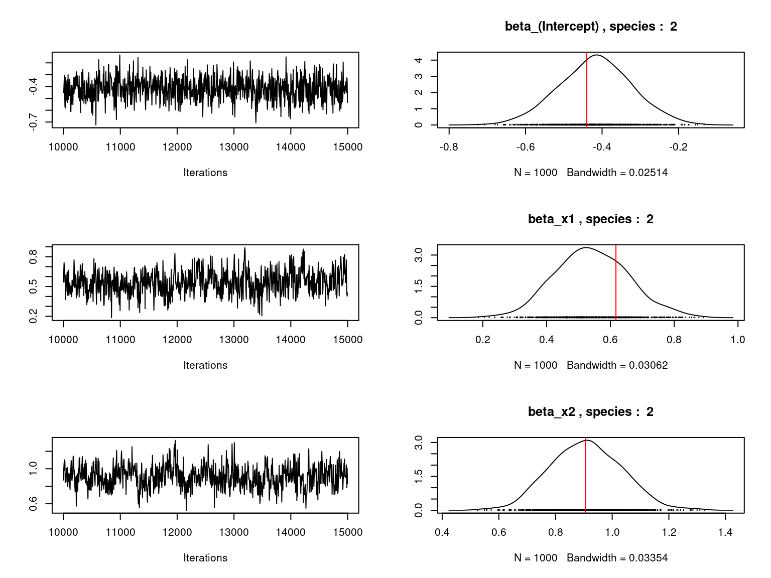
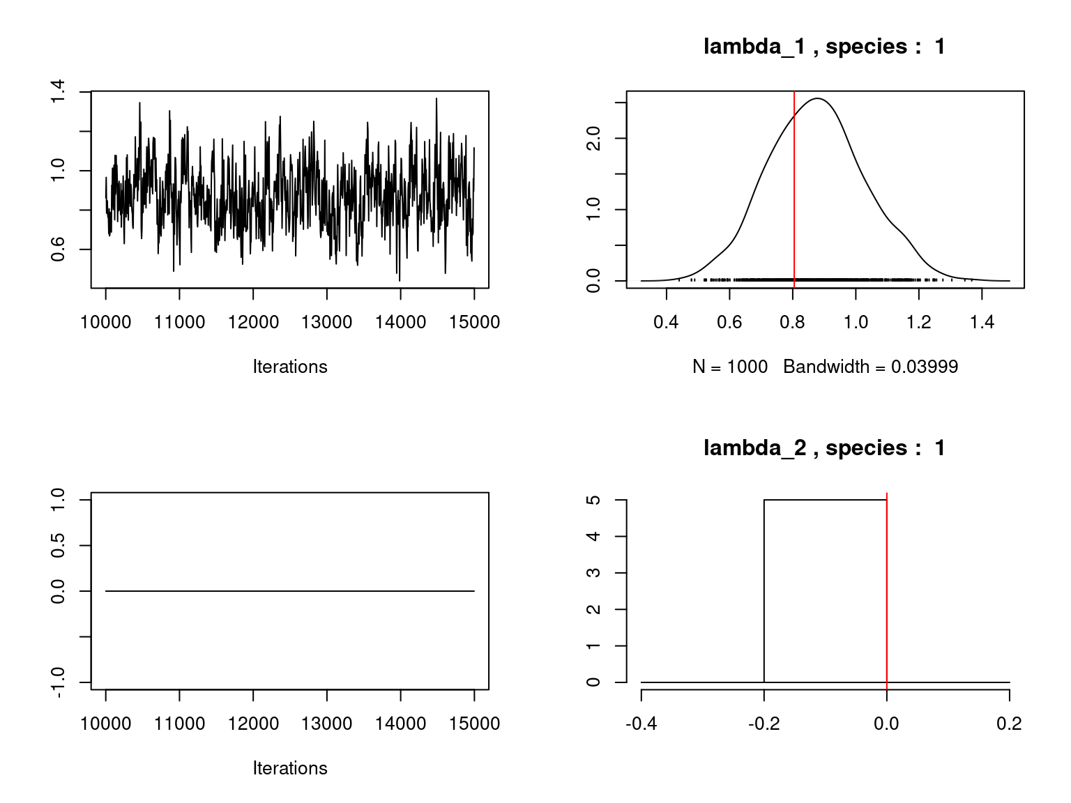
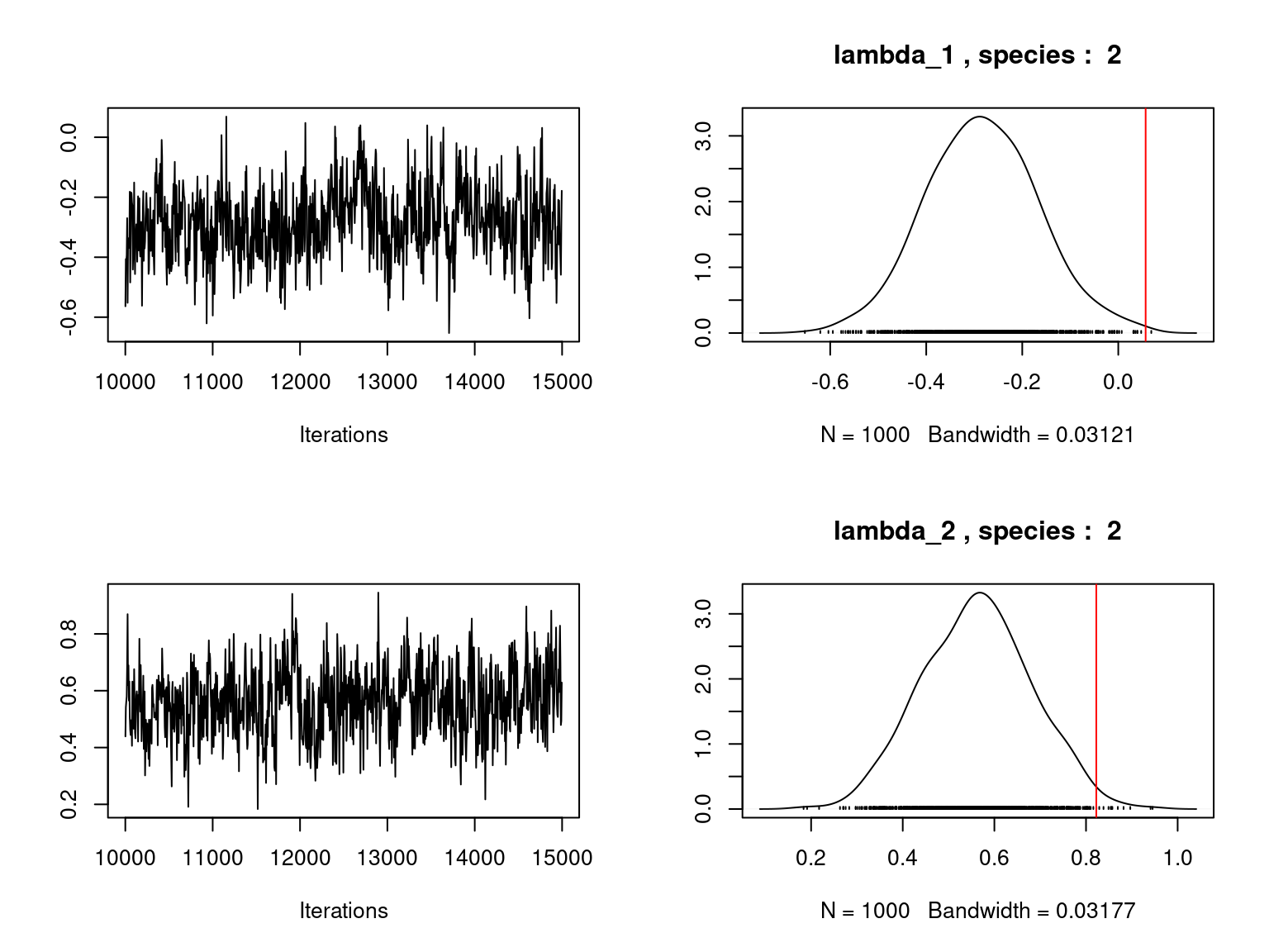
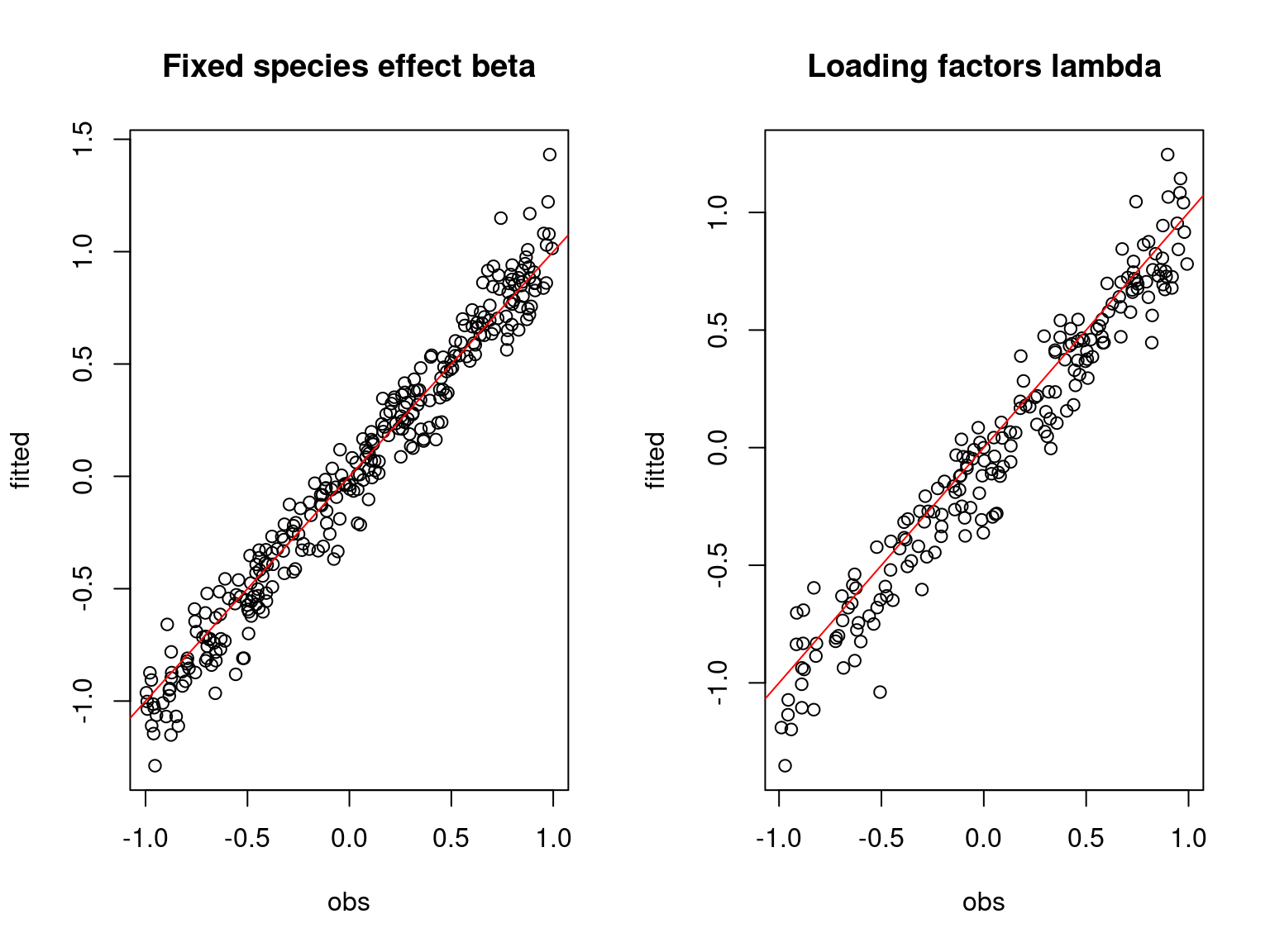
file="boral_simulation.RData")We visually evaluate the convergence of MCMCs by representing the trace and density a posteriori of some estimated parameters using the boral package and we plot the estimated parameters according to the expected ones to assess the accuracy of the package boral results.
load(file="jSDM_boral_cache/boral_simulation.RData")
mcmcsamps <- boral::get.mcmcsamples(mod_boral_sim)
boral_mcmc_beta0 <- mcmcsamps[,grep("lv.coefs\\[[1-9][0-9]?[0-9]?,1\\]", colnames(mcmcsamps))]
colnames(boral_mcmc_beta0) <- gsub(",1\\]",",0\\]",
gsub("lv.coefs", "X.coefs",
colnames(boral_mcmc_beta0)))
boral_mcmc_beta <- cbind(boral_mcmc_beta0,
mcmcsamps[,grep("X.coefs", colnames(mcmcsamps))])
boral_mcmc_lambda <- mcmcsamps[, grep("lv.coefs\\[[1-9][0-9]?[0-9]?,1\\]",
grep("lv.coefs", colnames(mcmcsamps),
value=TRUE), invert=TRUE, value=TRUE)]
## Fixed species effect beta for first two species
np <- ncol(X)
par(mfrow=c(ncol(X),2))
for (j in 1:2) {
for (p in 1:ncol(X)) {
coda::traceplot(coda::as.mcmc(boral_mcmc_beta[,j + nsp*(p-1)]))
coda::densplot(coda::as.mcmc(boral_mcmc_beta[,j + nsp*(p-1)]),
main=colnames(boral_mcmc_beta)[j + nsp*(p-1)])
abline(v=beta.target[p,j],col='red')
}
}
## Factor loadings lambda for first two species
par(mfrow=c(nl,2))
for (j in 1:2) {
for (l in 1:nl) {
coda::traceplot(coda::as.mcmc(boral_mcmc_lambda[,j + nsp*(l-1)]))
coda::densplot(coda::as.mcmc(boral_mcmc_lambda[,j + nsp*(l-1)]),
main=colnames(boral_mcmc_lambda)[j + nsp*(l-1)])
abline(v=lambda.target[l,j],col='red')
}
}
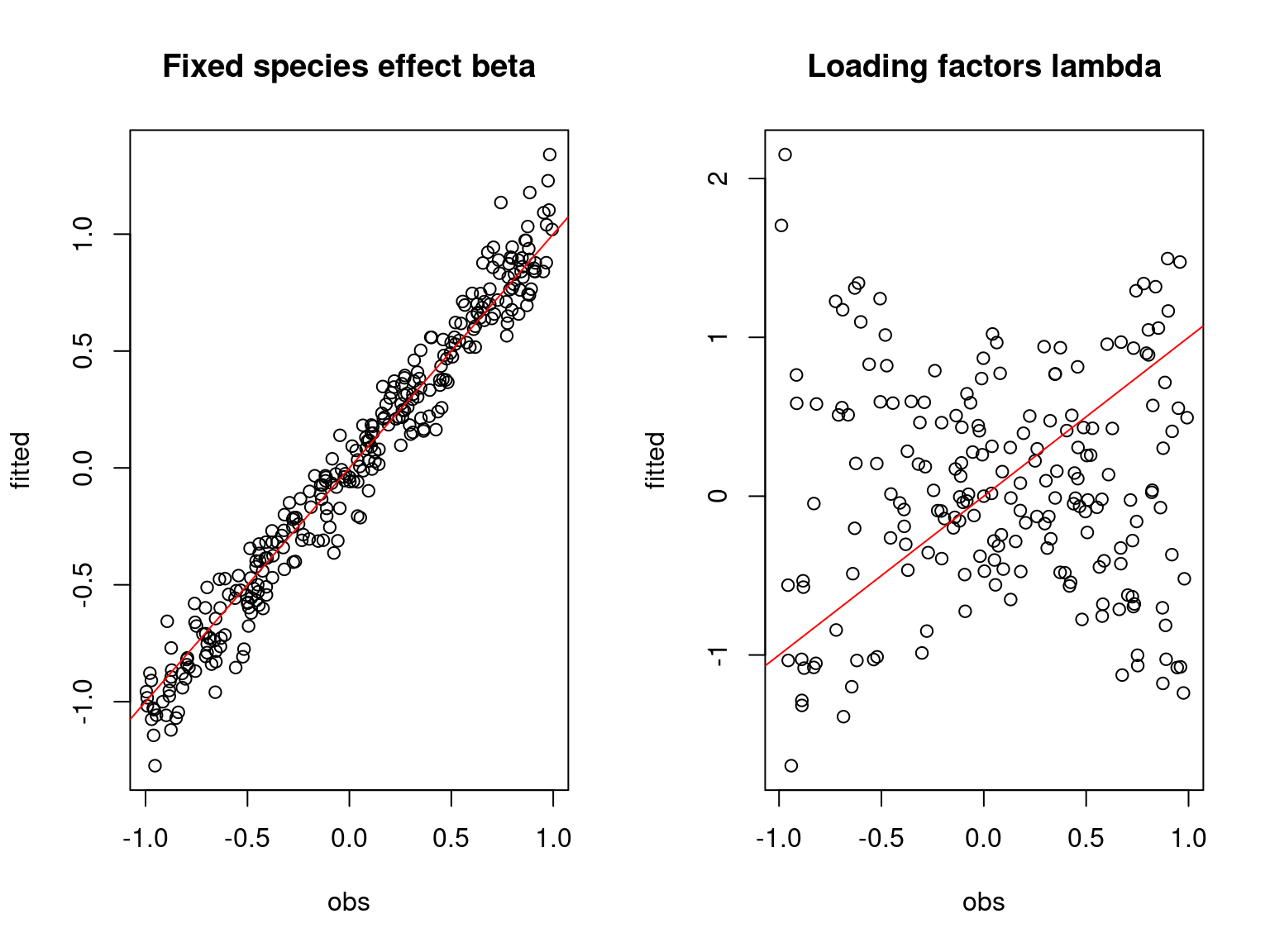
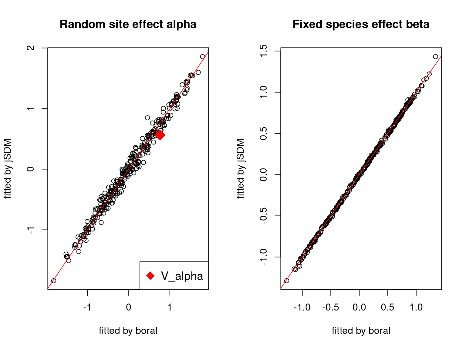
## Fixed species effect beta
par(mfrow=c(1,2))
plot(t(beta.target),
cbind(mod_boral_sim$lv.coefs.mean[,1],mod_boral_sim$X.coefs.mean),
xlab="obs", ylab="fitted", main="Fixed species effect beta")
abline(a=0,b=1,col='red')
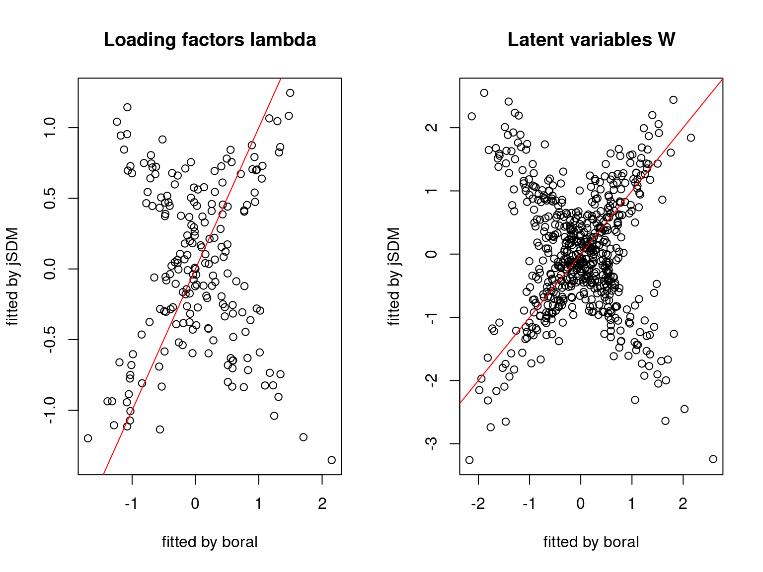
## factor loadings lambda_j
plot(t(lambda.target),mod_boral_sim$lv.coefs.mean[,-1],
xlab="obs", ylab="fitted", main="Loading factors lambda")
abline(a=0,b=1,col='red')
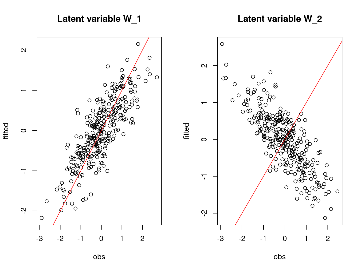
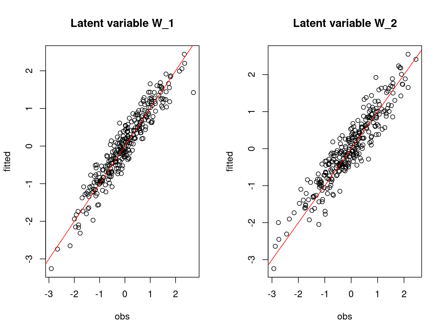
## Latent variable W
par(mfrow=c(1,2))
for (l in 1:nl) {
plot(W[,l],mod_boral_sim$lv.mean[,l],
main=paste0("Latent variable W_", l),
xlab="obs", ylab="fitted")
abline(a=0,b=1,col='red')
}
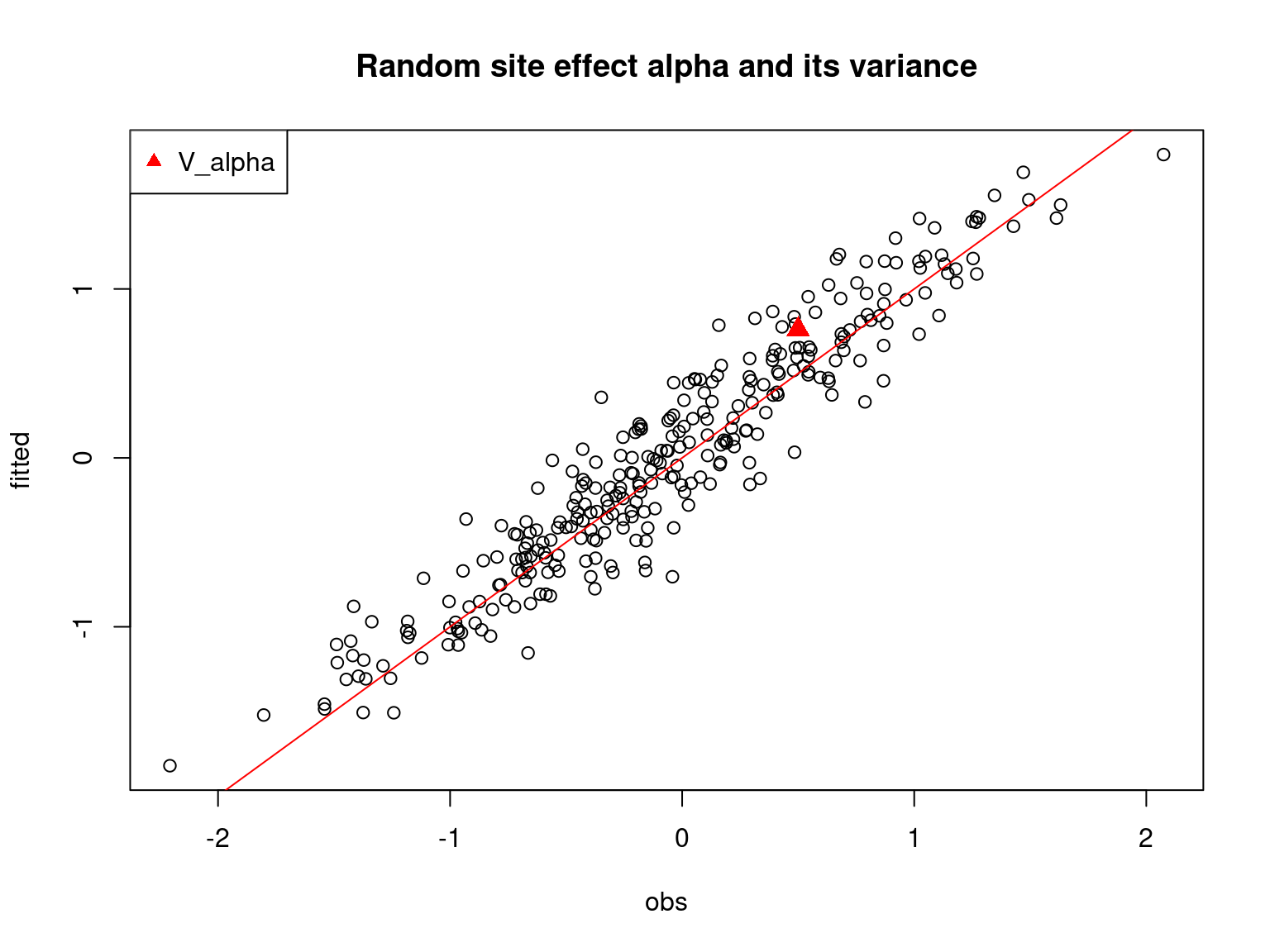
## alpha
par(mfrow=c(1,1))
plot(alpha.target, mod_boral_sim$row.coefs$ID1$mean,
xlab="obs", ylab="fitted")
abline(a=0,b=1,col='red')
points(V_alpha.target, mod_boral_sim$row.sigma$ID1["mean"],
pch=17, col='red', cex=1.5)
legend("topleft", legend="V_alpha", pch=17, col='red')
title("Random site effect alpha and its variance")
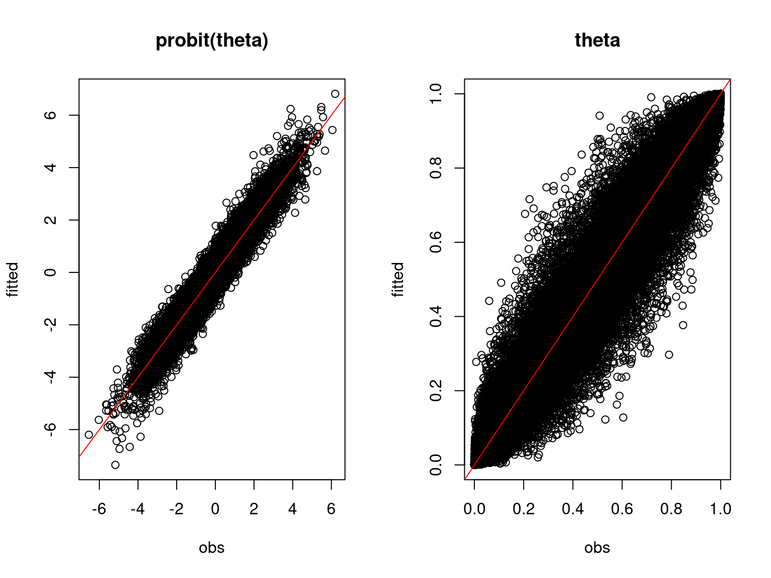
## Prediction
par(mfrow=c(1,2))
# probit_theta_latent
plot(probit_theta,probit_theta_latent_sim,
main="probit(theta)", xlab ="obs", ylab="fitted")
abline(a=0,b=1,col='red')
# theta_latent
plot(pnorm(probit_theta), pnorm(probit_theta_latent_sim),
main="theta", xlab ="obs", ylab="fitted")
abline(a=0,b=1,col='red')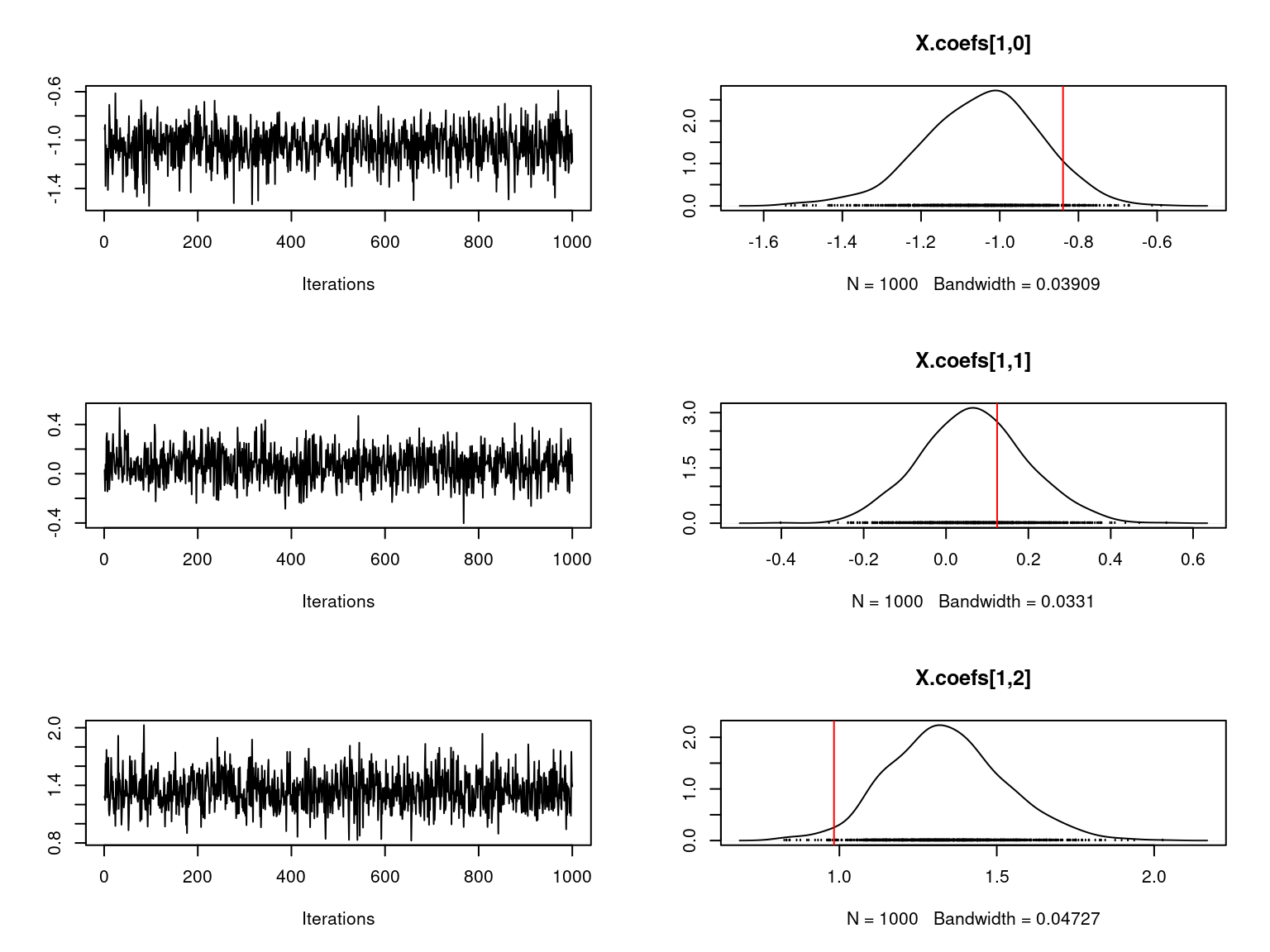

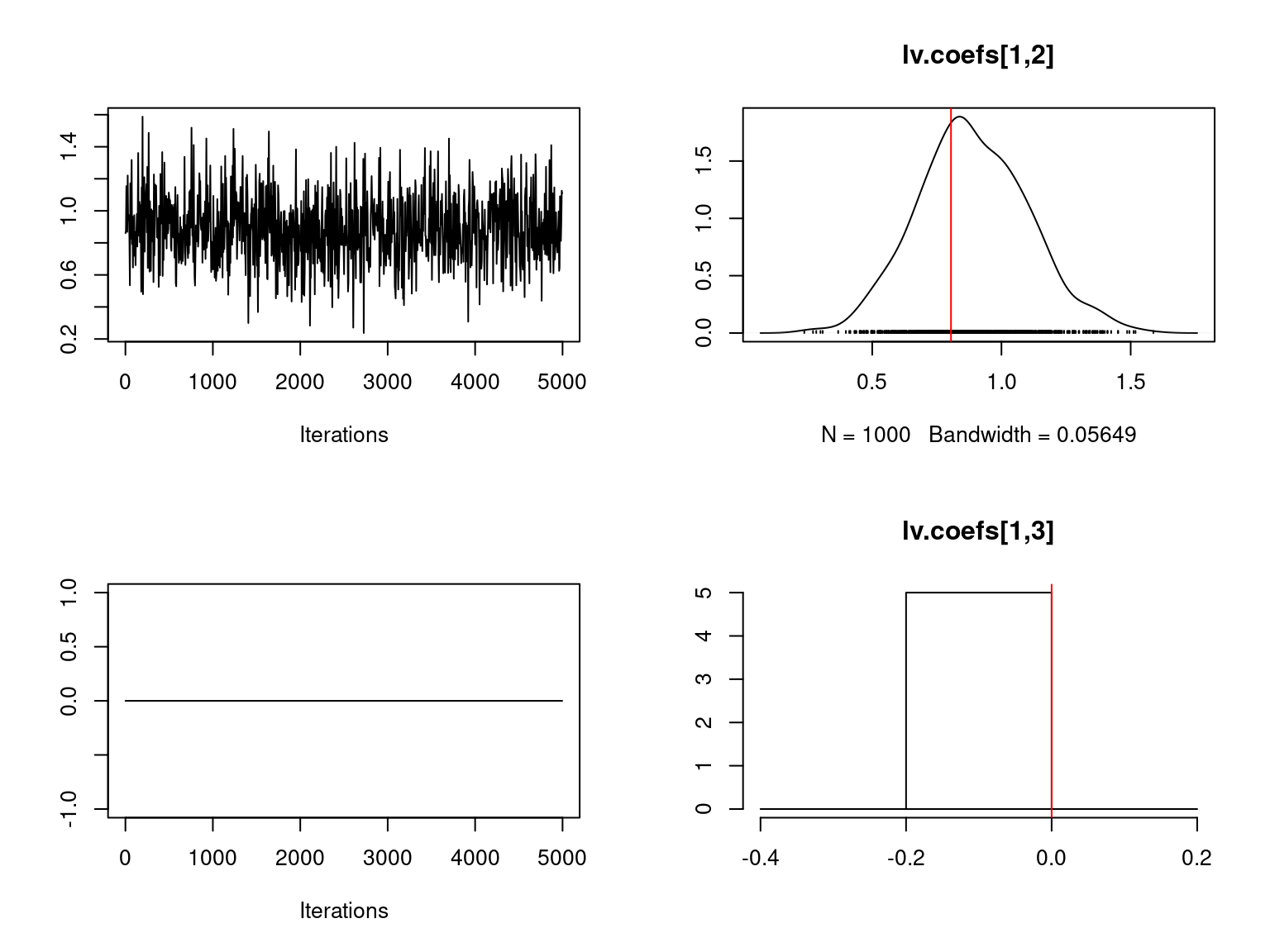
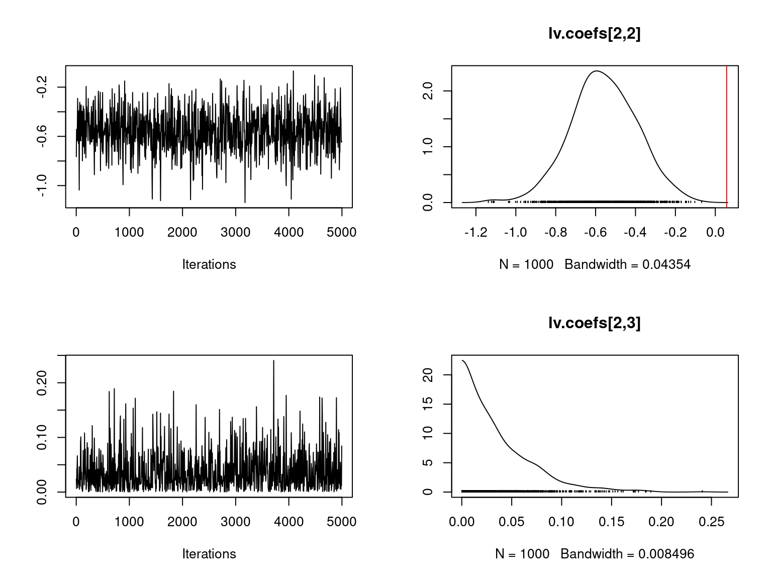
Overall, the traces and the densities of the parameters indicate the convergence of the algorithm. Indeed, we observe on the traces that the values oscillate around averages without showing an upward or downward trend and we see that the densities are quite smooth and for the most part of Gaussian form.
On the above figures, the estimated parameters are close to the expected values if the points are near the red line representing the identity function (\(y=x\)).
3.2 Mosquitos dataset
We fit a binomial joint species distribution model, including random site effect and latent variables, from the mosquitos data-set using boral() function to perform binomial probit regression.
setwd(paste0(dirname(rstudioapi::getSourceEditorContext()$path),"/jSDM_boral_cache"))
# Import center and reduce Mosquito data-set
data(mosquitos, package="jSDM")
head(mosquitos)
Env_Mosquitos <- mosquitos[,17:29]
Env_Mosquitos <- cbind(scale(Env_Mosquitos[,1:4]), Env_Mosquitos[,5:13])
PA_Mosquitos <- mosquitos[,1:16]

# Fit the model
T1 <- Sys.time()
mod_boral_Mosquitos <- boral(y=PA_Mosquitos, X=Env_Mosquitos,
                             save.model=TRUE, model.name="Mosquitos_jagsboralmodel.txt",
                             lv.control=list(num.lv=2), family="binomial",
                             prior.control = list(type=c("normal","normal",
                                                         "normal","uniform"),
                                            hypparams = c(10, 10, 10, 30)),
                             row.eff="random",
                             mcmc.control=list(n.burnin=10000,n.iteration=15000,
                                               n.thin=5,seed=123))
T2 <- Sys.time()
T_boral_Mosquitos <- difftime(T2,T1)

# Predicted probit(theta)
probit_theta_latent_Mosquitos <- mod_boral_Mosquitos$row.coefs[[1]]$mean +
  as.matrix(Env_Mosquitos) %*% t(mod_boral_Mosquitos$X.coefs.mean) +
  matrix(1,nrow=nrow(PA_Mosquitos), ncol=1)%*%mod_boral_Mosquitos$lv.coefs.mean[,"beta0"] +
  mod_boral_Mosquitos$lv.mean%*% t(mod_boral_Mosquitos$lv.coefs.mean[,-1])
# theta_latent
theta_latent_Mosquitos <- pnorm(probit_theta_latent_Mosquitos)
# Deviance
logL=0
for (i in 1:nrow(PA_Mosquitos)){
  for (j in 1:ncol(PA_Mosquitos)){
    logL=logL + dbinom(PA_Mosquitos[i,j],1,theta_latent_Mosquitos[i,j],1)
  }
}
Deviance_boral_Mosquitos <- -2*logL

save(T_boral_Mosquitos, mod_boral_Mosquitos,
     probit_theta_latent_Mosquitos, Deviance_boral_Mosquitos,
     file="boral_Mosquitos.RData")
3.3 Eucalypts dataset
We fit a binomial joint species distribution model, including random site effect and latent variables, from the eucalypts data-set using boral() function to perform binomial probit regression.
# Import center and reduce Eucalypts data-set
data(eucalypts, package="jSDM")
head(eucalypts)
Env_Eucalypts <- cbind(scale(eucalypts[,c("Rockiness","VallyBotFlat","PPTann", "cvTemp","T0")]),eucalypts[,c("Sandiness","Loaminess")])
PA_Eucalypts <- eucalypts[,1:12]
Env_Eucalypts <- Env_Eucalypts[rowSums(PA_Eucalypts) != 0,]
# Remove sites where none species was recorded
PA_Eucalypts <- PA_Eucalypts[rowSums(PA_Eucalypts) != 0,]

# Fit the model
T1 <- Sys.time()
mod_boral_Eucalypts <- boral(y=PA_Eucalypts, X=Env_Eucalypts,
                             save.model=TRUE, model.name="Eucalypts_jagsboralmodel.txt",
                             lv.control=list(num.lv=2), family="binomial",
                             prior.control=list(type=c("normal","normal",
                                                       "normal","uniform"),
                                                hypparams = c(10, 10, 10, 30)),
                             row.eff="random",
                             mcmc.control=list(n.burnin=10000,
                                               n.iteration=15000,
                                               n.thin=5, seed=123))
T2 <- Sys.time()
T_boral_Eucalypts <- difftime(T2,T1)

# Predicted probit(theta)
probit_theta_latent_Eucalypts <- mod_boral_Eucalypts$row.coefs[[1]]$mean +
  as.matrix(Env_Eucalypts) %*% t(mod_boral_Eucalypts$X.coefs.mean) +
  matrix(1,nrow=nrow(PA_Eucalypts),ncol=1)%*%mod_boral_Eucalypts$lv.coefs.mean[,"beta0"] +
  mod_boral_Eucalypts$lv.mean%*%t(mod_boral_Eucalypts$lv.coefs.mean[,-1])
# theta_latent
theta_latent_Eucalypts <- pnorm(probit_theta_latent_Eucalypts)
# Deviance
logL=0
for (i in 1:nrow(PA_Eucalypts)){
  for (j in 1:ncol(PA_Eucalypts)){
    logL=logL + dbinom(PA_Eucalypts[i,j],1,theta_latent_Eucalypts[i,j],1)
  }
}
Deviance_boral_Eucalypts <- -2*logL

save(T_boral_Eucalypts, mod_boral_Eucalypts,
     probit_theta_latent_Eucalypts, Deviance_boral_Eucalypts,
     file="boral_Eucalypts.RData")
3.4 Frogs dataset
We fit a binomial joint species distribution model, including random site effect and latent variables, from the frogs data-set using boral() function to perform binomial probit regression.
# Import center and reduce Frogs data-set
data(frogs, package="jSDM")
head(frogs)
Env_Frogs <- cbind(scale(frogs[,"Covariate_1"]),frogs[,"Covariate_2"],
                   scale(frogs[,"Covariate_3"]))
colnames(Env_Frogs) <- colnames(frogs[,1:3])
PA_Frogs <- frogs[,4:12]

# Fit the model
T1 <- Sys.time()
mod_boral_Frogs <- boral(y=PA_Frogs, X=Env_Frogs,
                         save.model=TRUE, model.name="Frogs_jagsboralmodel.txt",
                         lv.control=list(num.lv=2), family="binomial",
                         prior.control=list(type=c("normal","normal",
                                                   "normal","uniform"),
                                            hypparams = c(10, 10, 10, 30)),
                         row.eff="random",
                         mcmc.control=list(n.burnin=10000,
                                           n.iteration=15000,
                                           n.thin=5, seed=123))
T2 <- Sys.time()
T_boral_Frogs <- difftime(T2,T1)

# Predicted probit(theta)
probit_theta_latent_Frogs <- mod_boral_Frogs$row.coefs[[1]]$mean +
  as.matrix(Env_Frogs) %*% t(mod_boral_Frogs$X.coefs.mean) +
  matrix(1,nrow=nrow(PA_Frogs), ncol=1)%*%mod_boral_Frogs$lv.coefs.mean[,"beta0"] +
  mod_boral_Frogs$lv.mean%*%t(mod_boral_Frogs$lv.coefs.mean[,-1])
# theta_latent
theta_latent_Frogs <- pnorm(probit_theta_latent_Frogs)
# Deviance
logL=0
for (i in 1:nrow(PA_Frogs)){
  for (j in 1:ncol(PA_Frogs)){
    logL=logL + dbinom(PA_Frogs[i,j],1,theta_latent_Frogs[i,j],1)
  }
}
Deviance_boral_Frogs <- -2*logL

save(T_boral_Frogs, mod_boral_Frogs,
     probit_theta_latent_Frogs, Deviance_boral_Frogs,
     file="boral_Frogs.RData")
3.5 Fungi dataset
We fit a binomial joint species distribution model, including random site effect and latent variables, from the fungi data-set using boral() function to perform binomial probit regression.
# Import center and reduce fungi data-set
data(fungi, package="jSDM")
Env_Fungi <- cbind(scale(fungi[,c("diam","epi","bark")]),
                   fungi[,c("dc1","dc2","dc3","dc4","dc5",
                            "quality3","quality4","ground3","ground4")])
colnames(Env_Fungi) <- c("diam","epi","bark","dc1","dc2","dc3","dc4","dc5",
                         "quality3","quality4","ground3","ground4")
PA_Fungi <- fungi[,c("antser","antsin","astfer","fompin","hetpar","junlut",
                     "phefer","phenig","phevit","poscae","triabi")]
Env_Fungi <- Env_Fungi[rowSums(PA_Fungi) != 0,]
# Remove sites where none species was recorded
PA_Fungi<- PA_Fungi[rowSums(PA_Fungi) != 0,]

# Fit the model
T1 <- Sys.time()
mod_boral_Fungi <- boral(y=PA_Fungi, X=Env_Fungi,
                         save.model=TRUE, model.name="Fungi_jagsboralmodel.txt",
                         lv.control=list(num.lv=2), family="binomial",
                         prior.control=list(type=c("normal","normal",
                                                   "normal","uniform"),
                                            hypparams = c(10, 10, 10, 30)),
                         row.eff="random",
                         mcmc.control=list(n.burnin=10000,
                                           n.iteration=15000,
                                           n.thin=5, seed=123))
T2 <- Sys.time()
T_boral_Fungi <- difftime(T2,T1)

# Predicted probit(theta)
probit_theta_latent_Fungi <- mod_boral_Fungi$row.coefs[[1]]$mean +
  as.matrix(Env_Fungi) %*% t(mod_boral_Fungi$X.coefs.mean) +
  matrix(1,nrow=nrow(PA_Fungi), ncol=1)%*%mod_boral_Fungi$lv.coefs.mean[,"beta0"] +
  mod_boral_Fungi$lv.mean%*%t(mod_boral_Fungi$lv.coefs.mean[,-1])
# theta_latent
theta_latent_Fungi <- pnorm(probit_theta_latent_Fungi)
# Deviance
logL=0
for (i in 1:nrow(PA_Fungi)){
  for (j in 1:ncol(PA_Fungi)){
    logL=logL + dbinom(PA_Fungi[i,j],1,theta_latent_Fungi[i,j],1)
  }
}
Deviance_boral_Fungi <- -2*logL

save(T_boral_Fungi, mod_boral_Fungi,
     probit_theta_latent_Fungi, Deviance_boral_Fungi,
     file="boral_Fungi.RData")
3.6 Birds dataset
We fit a binomial joint species distribution model with multiple visit by site, including random site effect and latent variables, from the birds data-set using boral() function to perform binomial logistic regression.
We have to specify the JAGS model in the jagsboralmodel.txt file because the default JAGS model generated by boral function doesn’t allow to indicate different number of trials for each site as it is the case in birds data-set.
# Import center and reduce birds data-set
data(birds, package="jSDM")
# data.obs
PA_Birds <- birds[,1:158]
# Remove species with less than 5 presences
rare_sp <- which(apply(PA_Birds>0, 2, sum) < 5)
PA_Birds <- PA_Birds[, -rare_sp]
# Normalized continuous variables
Env_Birds <- data.frame(cbind(scale(birds[,c("elev","rlength","forest")]),
                              birds[,"nsurvey"]))
colnames(Env_Birds) <- c("elev","rlength","forest","nsurvey")
# Compute design matrix
mf.suit <- model.frame(formula=~elev+rlength+forest-1, data=Env_Birds)
X_Birds <- model.matrix(attr(mf.suit,"terms"), data=mf.suit)
# Number of latent variables
num.lv <- 2
# Fit the model
library(jagsUI)
T1 <- Sys.time()
# Number of trials by site impossible to specify with boral,
# trial.size either equal to a single element
# or a vector of length equal to the number of columns in y
# mod_boral_Birds <- boral(y=PA_Birds, X=X_Birds,
#                          lv.control=list(num.lv=2), family="binomial",
#                          save.model=TRUE, model.name="Birds_jagsboralmodel.txt",
#                          trial.size=max(Env_Birds$nsurvey),
#                          prior.control=list(type=c("normal","normal",
#                                                    "normal","uniform"),
#                                             hypparams = c(10, 10, 10, 30)),
#                          row.eff="random",
#                          mcmc.control=list(n.burnin=10000,
#                                            n.iteration=15000,
#                                            n.thin=5,seed=123))
# JAGS model in vignettes/jSDM_boral_cache/Birds_jagsboralmodel.txt
# modified to specify the number of trials by site
# Data needed to fit the model
jags.data <- list(y=as.matrix(PA_Birds), n=nrow(PA_Birds), p=ncol(PA_Birds),
                  X=as.matrix(X_Birds), visits=Env_Birds$nsurvey, num.lv = 2)
# Starting values
gen.inits <- function() {
    alpha <- rep(0,nrow(PA_Birds))
    Valpha <- 1
    beta <- matrix(0, ncol(PA_Birds), ncol(X_Birds))
    lambda <- matrix(0, ncol(PA_Birds),num.lv +1)
    for (j in 1:ncol(PA_Birds)){
      for (k in 1:num.lv){
        lambda[k,k+1] <- 1
        if(j<k) {
          lambda[j,k+1] <- NA
        }
      }
    }
    W <- matrix(0, nrow(PA_Birds), num.lv)
    list("X.coefs"=beta,"row.coefs"=alpha,"row.sigma"=Valpha,"lvs"=W, "lv.coefs" = lambda)
    }
# Fit JAGS model
mod_boral_Birds <- jagsUI::jags(data = jags.data, inits <- gen.inits,
                                parameters.to.save = c("X.coefs","row.coefs",
                                                       "row.sigma","lvs", "lv.coefs"),
                                model.file = "Birds_jagsboralmodel.txt",
                                n.chains = 1, n.iter=15000, n.burnin = 10000, n.thin = 5)
T2 <- Sys.time()
T_boral_Birds <- difftime(T2,T1)

# Predicted logit(theta)
logit_theta_latent_Birds <- c(mod_boral_Birds$mean$row.coefs) +
  as.matrix(X_Birds) %*% t(as.matrix(mod_boral_Birds$mean$X.coefs)) +
  matrix(1,nrow=nrow(PA_Birds), ncol=1)%*% mod_boral_Birds$mean$lv.coefs[,1] +
  mod_boral_Birds$mean$lvs%*%t(mod_boral_Birds$mean$lv.coefs[,-1])
# theta_latent
theta_latent_Birds <- inv_logit(logit_theta_latent_Birds)
# Deviance
logL=0
for (i in 1:nrow(PA_Birds)){
  for (j in 1:ncol(PA_Birds)){
    logL= logL + dbinom(PA_Birds[i,j],Env_Birds$nsurvey[i],theta_latent_Birds[i,j],1)
  }
}
Deviance_boral_Birds <- -2*logL
# mod_boral_Birds$mean$deviance
save(T_boral_Birds, mod_boral_Birds,
     logit_theta_latent_Birds, Deviance_boral_Birds,
     file="boral_Birds.RData")
3.7 Mites dataset
We fit a joint species distribution model, including random site effect and latent variables, from the mites abundance data-set using boral() function to perform a poisson log-linear regression.
# Import center and reduce mites data-set
data(mites, package="jSDM")
# data.obs
PA_Mites <- mites[,1:35]
# Remove species with less than 10 presences
rare_sp <- which(apply(PA_Mites>0, 2, sum) < 10)
PA_Mites <- PA_Mites[, -rare_sp]
# Normalized continuous variables
Env_Mites  <- cbind(scale(mites[,c("density","water")]),
                    mites[,c("substrate", "shrubs", "topo")])
mf.suit <- model.frame(formula=~., data=as.data.frame(Env_Mites))
X_Mites <- model.matrix(attr(mf.suit,"terms"), data=mf.suit)
# Fit the model
T1 <- Sys.time()
mod_boral_Mites <- boral(y=PA_Mites, X=X_Mites[,-1],
                         save.model=TRUE, model.name="Mites_jagsboralmodel.txt",
                         lv.control=list(num.lv=2), family="poisson",
                         prior.control=list(type=c("normal","normal",
                                                   "normal","uniform"),
                                            hypparams = c(10, 10, 10, 30)),
                         row.eff="random",
                         mcmc.control=list(n.burnin=10000,
                                           n.iteration=15000,
                                           n.thin=5, seed=123))
T2 <- Sys.time()
T_boral_Mites <- difftime(T2,T1)

# Predicted probit(theta)
log_theta_latent_Mites <- as.matrix(X_Mites[,-1]) %*% t(mod_boral_Mites$X.coefs.mean) +
  matrix(1,nrow=nrow(PA_Mites), ncol=1)%*%mod_boral_Mites$lv.coefs.mean[,"beta0"] +
  mod_boral_Mites$lv.mean%*%t(mod_boral_Mites$lv.coefs.mean[,-1]) +
  c(mod_boral_Mites$row.coefs[[1]]$mean)
# theta_latent
theta_latent_Mites <- exp(log_theta_latent_Mites)
# Deviance
logL=0
for (i in 1:nrow(PA_Mites)){
  for (j in 1:ncol(PA_Mites)){
    logL=logL + dpois(PA_Mites[i,j],theta_latent_Mites[i,j],1)
  }
}
Deviance_boral_Mites <- -2*logL

save(T_boral_Mites, mod_boral_Mites,
     log_theta_latent_Mites, Deviance_boral_Mites,
     file="boral_Mites.RData")
4 Package jSDM
In a second step, we fit the same joint species distribution models from each of the previous data-sets using the jSDM package.
4.1 Simulated dataset
We fit a binomial joint species distribution model, including random site effect and latent variables, from the simulated data-set using the jSDM_binomial_probit() function to perform binomial probit regression.
setwd(dirname(rstudioapi::getSourceEditorContext()$path))
load(file="jSDM_boral_cache/boral_simulation.RData")
library(jSDM)
# Fit the model
T1<-Sys.time()
mod_jSDM_sim <- jSDM_binomial_probit(
  # Chains
  burnin=10000, mcmc=5000, thin=5,
  # Response variable
  presence_data=Y,
  # Explanatory variables
  site_formula=~x1+x2,
  site_data=X,
  # Model specification
  n_latent=2, site_effect="random",
  # Starting values
  alpha_start=0, beta_start=0,
  lambda_start=0, W_start=0,
  V_alpha=1,
  # Priors
  shape_Valpha=0.1,
  rate_Valpha=0.1,
  mu_beta=0, V_beta=10,
  mu_lambda=0, V_lambda=10,
  # Various
  seed=123, verbose=1)
T2<-Sys.time()
T_jSDM_sim=difftime(T2, T1)

# RMSE
SE=(pnorm(probit_theta)-mod_jSDM_sim$theta_latent)^2
RMSE_jSDM_sim=sqrt(sum(SE/(nsite*nsp)))

save(T_jSDM_sim, mod_jSDM_sim, RMSE_jSDM_sim,
     file="jSDM_boral_cache/jSDM_simulation.RData")
We visually evaluate the convergence of MCMCs by representing the trace and density a posteriori of some estimated parameters using the jSDM package and we plot the estimated parameters according to the expected ones to assess the accuracy of the package jSDM results.
load(file="jSDM_boral_cache/jSDM_simulation.RData")
# ===================================================
# Result analysis
# ===================================================

## Fixed species effect beta for first two species
np <- ncol(X)
mean_beta <- matrix(0,nsp,np)
par(mfrow=c(ncol(X),2))
for (j in 1:nsp) {
  for (p in 1:ncol(X)) {
    mean_beta[j,p] <-mean(mod_jSDM_sim$mcmc.sp[[j]][,p])
    if (j < 3){
      coda::traceplot(coda::as.mcmc(mod_jSDM_sim$mcmc.sp[[j]][,p]))
      coda::densplot(coda::as.mcmc(mod_jSDM_sim$mcmc.sp[[j]][,p]),
                     main=paste(colnames(mod_jSDM_sim$mcmc.sp
                                         [[j]])[p],", species : ",j))
      abline(v=beta.target[p,j],col='red')
    }
  }
}

## Factor loadings lambda_j for first two species
mean_lambda <- matrix(0,nsp,nl)
par(mfrow=c(nl,2))
for (j in 1:nsp) {
  for (l in 1:nl) {
    mean_lambda[j,l] <-mean(mod_jSDM_sim$mcmc.sp[[j]][,ncol(X)+l])

    if (j < 3){
      coda::traceplot(coda::as.mcmc(mod_jSDM_sim$mcmc.sp[[j]][,ncol(X)+l]))
      coda::densplot(coda::as.mcmc(mod_jSDM_sim$mcmc.sp[[j]][,ncol(X)+l]),
                     main=paste(colnames(mod_jSDM_sim$mcmc.sp
                                         [[j]])[ncol(X)+l],", species : ",j))
      abline(v=lambda.target[l,j],col='red')
    }
  }
}

# Fixed species effects
par(mfrow=c(1,2))
plot(t(beta.target),mean_beta, xlab="obs", ylab="fitted",
     main="Fixed species effect beta")
abline(a=0,b=1,col='red')
plot(t(lambda.target),mean_lambda, xlab="obs", ylab="fitted",
     main="Loading factors lambda")
abline(a=0,b=1,col='red')

## W latent variables
par(mfrow=c(1,2))
for (l in 1:nl) {
  plot(W[,l],apply(mod_jSDM_sim$mcmc.latent[[paste0("lv_",l)]],2,mean),
       main=paste0("Latent variable W_", l), xlab="obs", ylab="fitted")
  abline(a=0,b=1,col='red')
}

## V_alpha
par(mfrow=c(1,2))
coda::traceplot(mod_jSDM_sim$mcmc.V_alpha, main="V_alpha")
coda::densplot(mod_jSDM_sim$mcmc.V_alpha, main="V_alpha")
abline(v=V_alpha.target,col='red')

## alpha
par(mfrow=c(1,1))
plot(alpha.target,apply(mod_jSDM_sim$mcmc.alpha,2,mean),
     xlab= "obs", ylab="fitted", main="Random site effect alpha")
abline(a=0,b=1,col='red')

## Deviance
plot(mod_jSDM_sim$mcmc.Deviance, main="Deviance")

#= Predictions
## probit_theta
par(mfrow=c(1,2))
plot(probit_theta,mod_jSDM_sim$probit_theta_latent,
     xlab="obs",ylab="fitted", main="probit(theta)")
abline(a=0,b=1,col='red')
## theta
plot(pnorm(probit_theta),mod_jSDM_sim$theta_latent,
     xlab="obs",ylab="fitted", main="theta")
abline(a=0,b=1,col='red')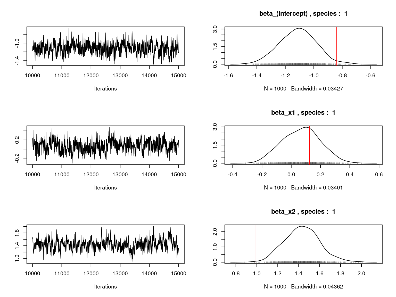
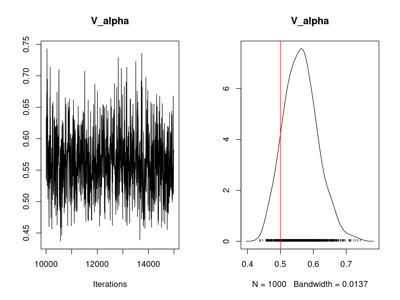
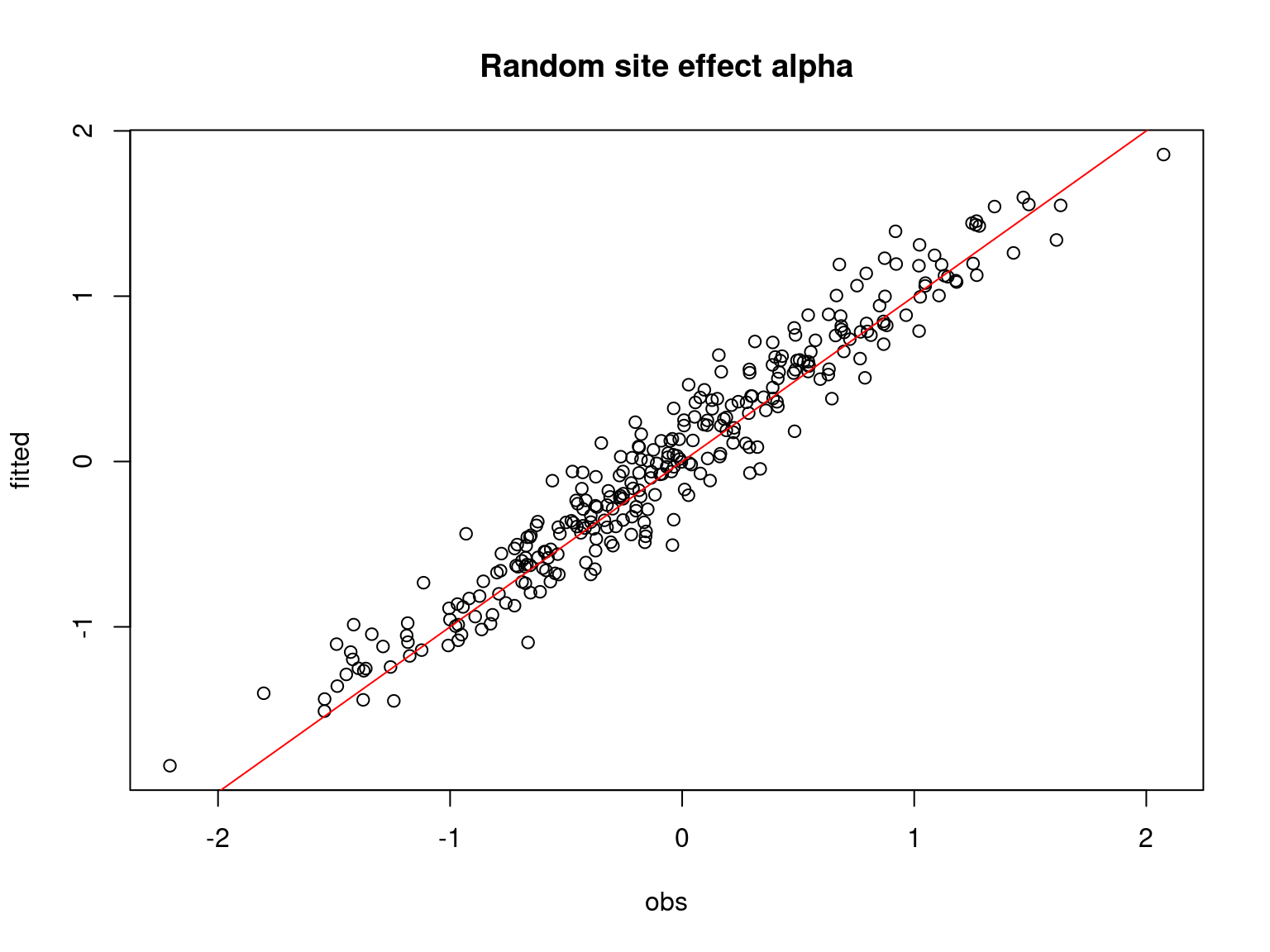
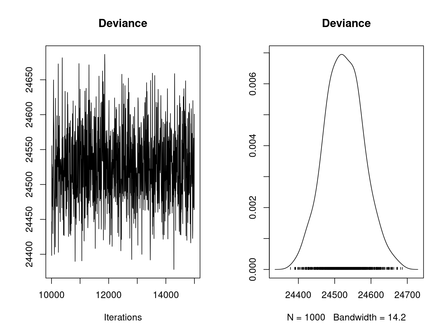
Overall, the traces and the densities of the parameters indicate the convergence of the algorithm. Indeed, we observe on the traces that the values oscillate around averages without showing an upward or downward trend and we see that the densities are quite smooth and for the most part of Gaussian form.
On the above figures, the estimated parameters are close to the expected values if the points are near the red line representing the identity function (\(y=x\)).
4.2 Mosquitos dataset
We fit a binomial joint species distribution model, including random site effect and latent variables, from the mosquitos data-set using jSDM_binomial_probit() function to perform binomial probit regression.
# Fit the model
T1 <- Sys.time()
mod_jSDM_Mosquitos <- jSDM_binomial_probit(
  # Chains
  burnin=10000, mcmc=5000, thin=5,
  # Response variable
  presence_data=PA_Mosquitos,
  # Explanatory variables
  site_formula=~.,
  site_data=Env_Mosquitos,
  # Model specification
  site_effect="random", n_latent=2,
  # Starting values
  alpha_start=0, beta_start=0,
  lambda_start=0, W_start=0,
  V_alpha=1,
  # Priors
  shape_Valpha=0.1,
  rate_Valpha=0.1,
  mu_beta=0, V_beta=10 ,
  mu_lambda=0, V_lambda=10,
  # Various
  seed=123, verbose=1)
T2 <- Sys.time()
T_jSDM_Mosquitos <- difftime(T2,T1)
save(T_jSDM_Mosquitos, mod_jSDM_Mosquitos,
     file="jSDM_boral_cache/jSDM_Mosquitos.RData")
4.3 Eucalypts dataset
We fit a binomial joint species distribution model, including random site effect and latent variables, from the eucalypts data-set using jSDM_binomial_probit() function to perform binomial probit regression.
# Fit the model
T1 <- Sys.time()
mod_jSDM_Eucalypts <- jSDM_binomial_probit(
  # Chains
  burnin=10000, mcmc=5000, thin=5,
  # Response variable
  presence_data=PA_Eucalypts,
  # Explanatory variables
  site_formula=~.,
  site_data=Env_Eucalypts,
  # Model specification
  n_latent=2, site_effect="random",
  # Starting values
  alpha_start=0, beta_start=0,
  lambda_start=0, W_start=0,
  V_alpha=1,
  # Priors
  shape_Valpha=0.1,
  rate_Valpha=0.1,
  mu_beta=0, V_beta=10 ,
  mu_lambda=0, V_lambda=10,
  # Various
  seed=123, verbose=1)
T2 <- Sys.time()
T_jSDM_Eucalypts <- difftime(T2,T1)
save(T_jSDM_Eucalypts, mod_jSDM_Eucalypts,
     file="jSDM_boral_cache/jSDM_Eucalypts.RData")
4.4 Frogs dataset
We fit a binomial joint species distribution model, including random site effect and latent variables, from the frogs data-set using jSDM_binomial_probit() function to perform binomial probit regression.
# Fit the model
T1 <- Sys.time()
mod_jSDM_Frogs <- jSDM_binomial_probit(
  # Chains
  burnin=10000, mcmc=5000, thin=5,
  # Response variable
  presence_data=as.matrix(PA_Frogs),
  # Explanatory variables
  site_formula=~.,
  site_data=as.data.frame(Env_Frogs),
  # Model specification
  n_latent=2, site_effect="random",
  # Starting values
  alpha_start=0, beta_start=0,
  lambda_start=0, W_start=0,
  V_alpha=1,
  # Priors
  shape_Valpha=0.1,
  rate_Valpha=0.1,
  mu_beta=0, V_beta=10,
  mu_lambda=0, V_lambda=10,
  # Various
  seed=123, verbose=1)
T2 <- Sys.time()
T_jSDM_Frogs <- difftime(T2,T1)
save(T_jSDM_Frogs, mod_jSDM_Frogs,
     file="jSDM_boral_cache/jSDM_Frogs.RData")
4.5 Fungi dataset
We fit a binomial joint species distribution model, including random site effect and latent variables, from the fungi data-set using jSDM_binomial_probit() function to perform binomial probit regression.
# Fit the model
T1 <- Sys.time()
mod_jSDM_Fungi <- jSDM_binomial_probit(
  # Chains
  burnin=10000, mcmc=5000, thin=5,
  # Response variable
  presence_data=PA_Fungi,
  # Explanatory variables
  site_formula=~.,
  site_data=Env_Fungi,
  # Model specification
  n_latent=2, site_effect="random",
  # Starting values
  alpha_start=0, beta_start=0,
  lambda_start=0, W_start=0,
  V_alpha=1,
  # Priors
  shape_Valpha=0.1,
  rate_Valpha=0.1,
  mu_beta=0, V_beta=10,
  mu_lambda=0, V_lambda=10,
  # Various
  seed=123, verbose=1)
T2 <- Sys.time()
T_jSDM_Fungi <- difftime(T2,T1)
save(T_jSDM_Fungi, mod_jSDM_Fungi,
     file="jSDM_boral_cache/jSDM_Fungi.RData")
4.6 Birds dataset
We fit a binomial joint species distribution model with multiple visit by site, including random site effect and latent variables, from the birds data-set using jSDM_binomial_logit() function to perform binomial logistic regression.
# Fit the model
T1 <- Sys.time()
mod_jSDM_Birds <- jSDM_binomial_logit(
  # Chains
  burnin=10000, mcmc=5000, thin=5,
  # Response variable
  presence_data=PA_Birds,
  # Explanatory variables
  site_formula=~elev+rlength+forest,
  site_data=Env_Birds,
  trials= Env_Birds$nsurvey,
  # Model specification
  n_latent=2, site_effect="random",
  # Starting values
  alpha_start=0, beta_start=0,
  lambda_start=0, W_start=0,
  V_alpha=1,
  # Priors
  shape_Valpha=0.1,
  rate_Valpha=0.1,
  mu_beta=0, V_beta=10 ,
  mu_lambda=0, V_lambda=10,
  # Various
  ropt=0.44,
  seed=123, verbose=1)
T2 <- Sys.time()
T_jSDM_Birds <- difftime(T2,T1)
save(T_jSDM_Birds, mod_jSDM_Birds,
     file="jSDM_boral_cache/jSDM_Birds.RData")
4.7 Mites dataset
We fit a joint species distribution model, including random site effect and latent variables, from the mites abundance data-set using jSDM_poisson_log() function to perform a poisson log-linear regression.
# Fit the model
T1 <- Sys.time()
mod_jSDM_Mites <- jSDM_poisson_log(
  # Chains
  burnin=10000, mcmc=5000, thin=5,
  # Response variable
  count_data=PA_Mites,
  # Explanatory variables
  site_formula=~.,
  site_data=Env_Mites,
  # Model specification
  n_latent=2, site_effect="random",
  # Starting values
  alpha_start=0, beta_start=0,
  lambda_start=0, W_start=0,
  V_alpha=1,
  # Priors
  shape_Valpha=0.1,
  rate_Valpha=0.1,
  mu_beta=0, V_beta=10 ,
  mu_lambda=0, V_lambda=10,
  # Various
  ropt=0.44,
  seed=123, verbose=1)
T2 <- Sys.time()
T_jSDM_Mites <- difftime(T2,T1)
save(T_jSDM_Mites, mod_jSDM_Mites,
     file="jSDM_boral_cache/jSDM_Mites.RData")
5 Comparison
Then we compare the computation time and the results obtained with each package.
5.1 Computation time and deviance
| Simulated | Mosquitos | Eucalypts | Frogs | Fungi | Birds | Mites | |
|---|---|---|---|---|---|---|---|
| Computation time boral (secondes) | 35546 | 2175 | 1439 | 83 | 2369 | 3909 | 533 |
| Computation time jSDM (secondes) | 133 | 17 | 33 | 6 | 32 | 1164 | 109 |
| Deviance boral | 23255 | 1079 | 1703 | 120 | 1220 | 30193 | 6127 |
| Deviance jSDM | 23164 | 996 | 1598 | 101 | 1155 | 30133 | 6089 |
|
|
|
|
|
|
|
|
jSDM is 3 to 268 times faster than boral/JAGS.
5.2 Root-Mean-Square Error (RMSE) for simulated data
Computed for the probabilities of presences \(\theta_{ij}\) with the simulated data-set.
| boral | jSDM | |
|---|---|---|
| RMSE | 0.089 | 0.087 |
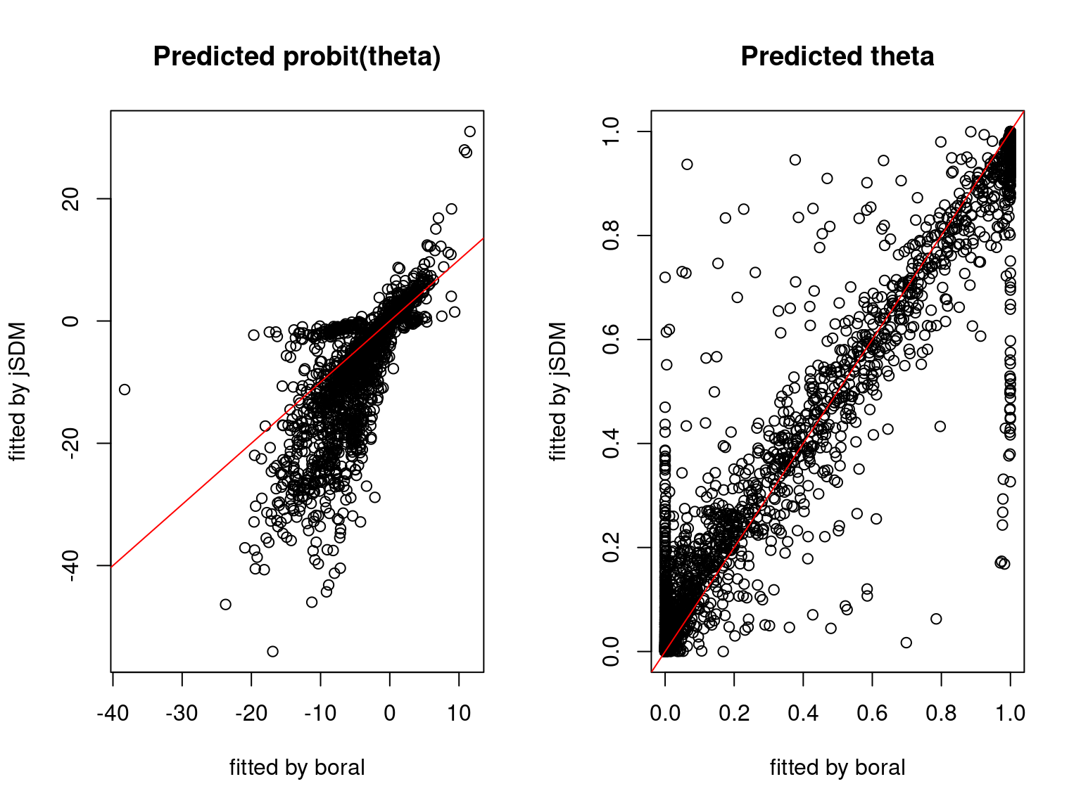
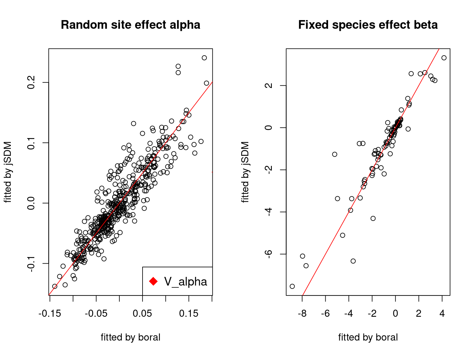
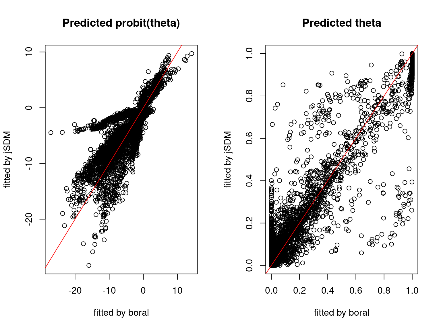
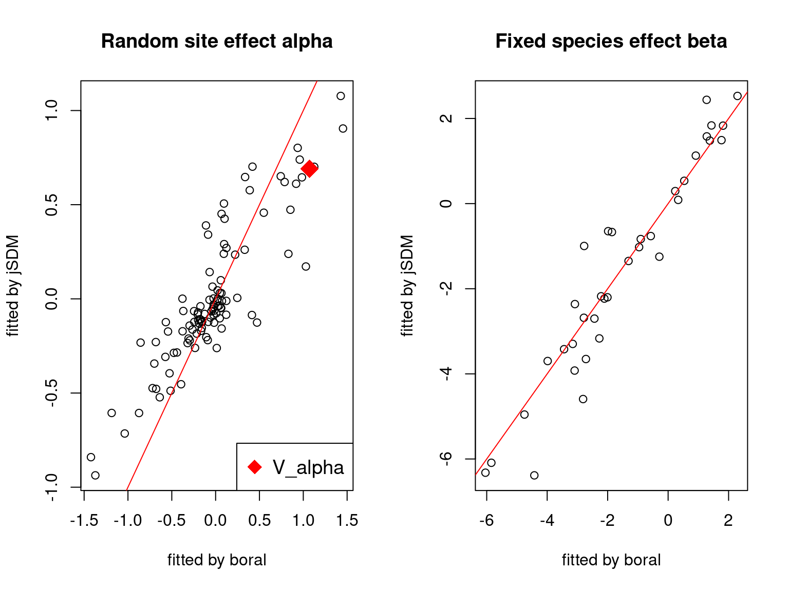
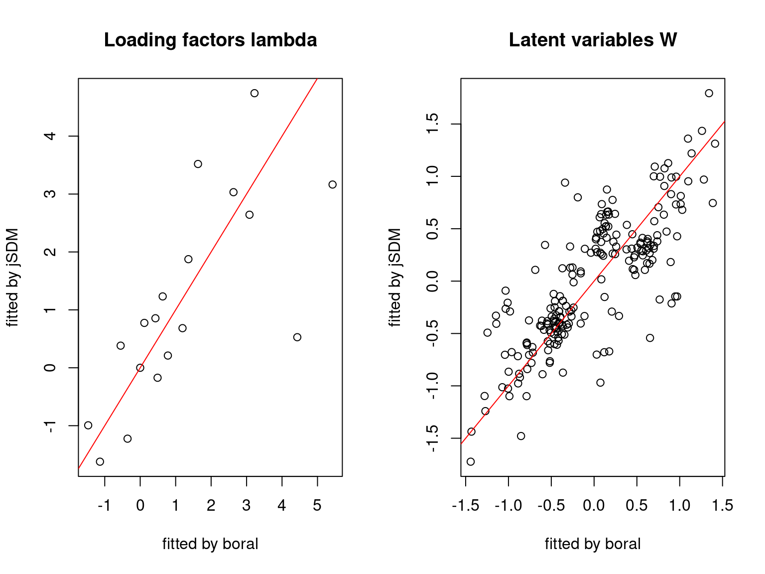
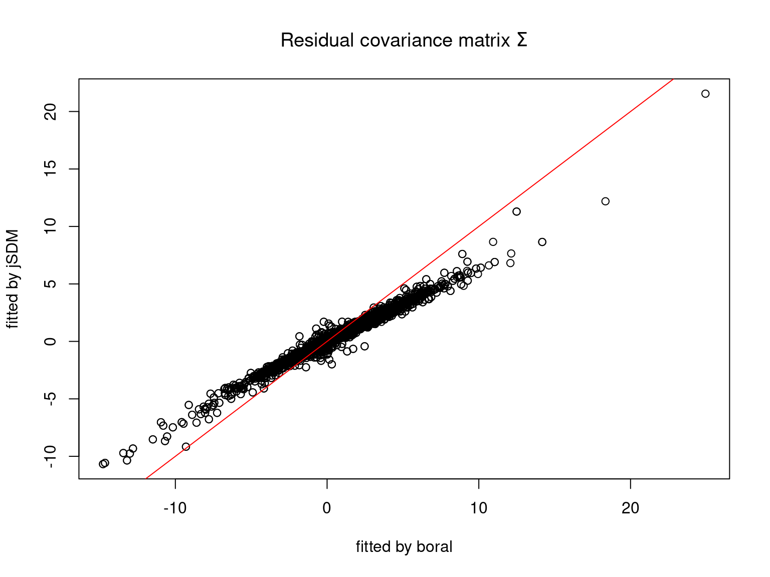
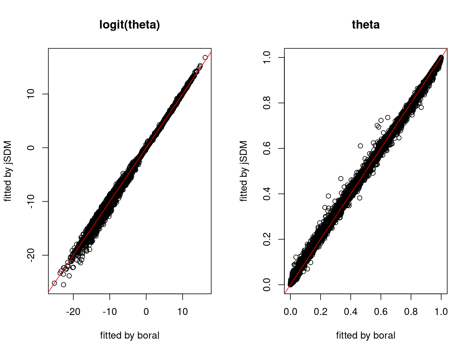
5.3 Estimated Parameters
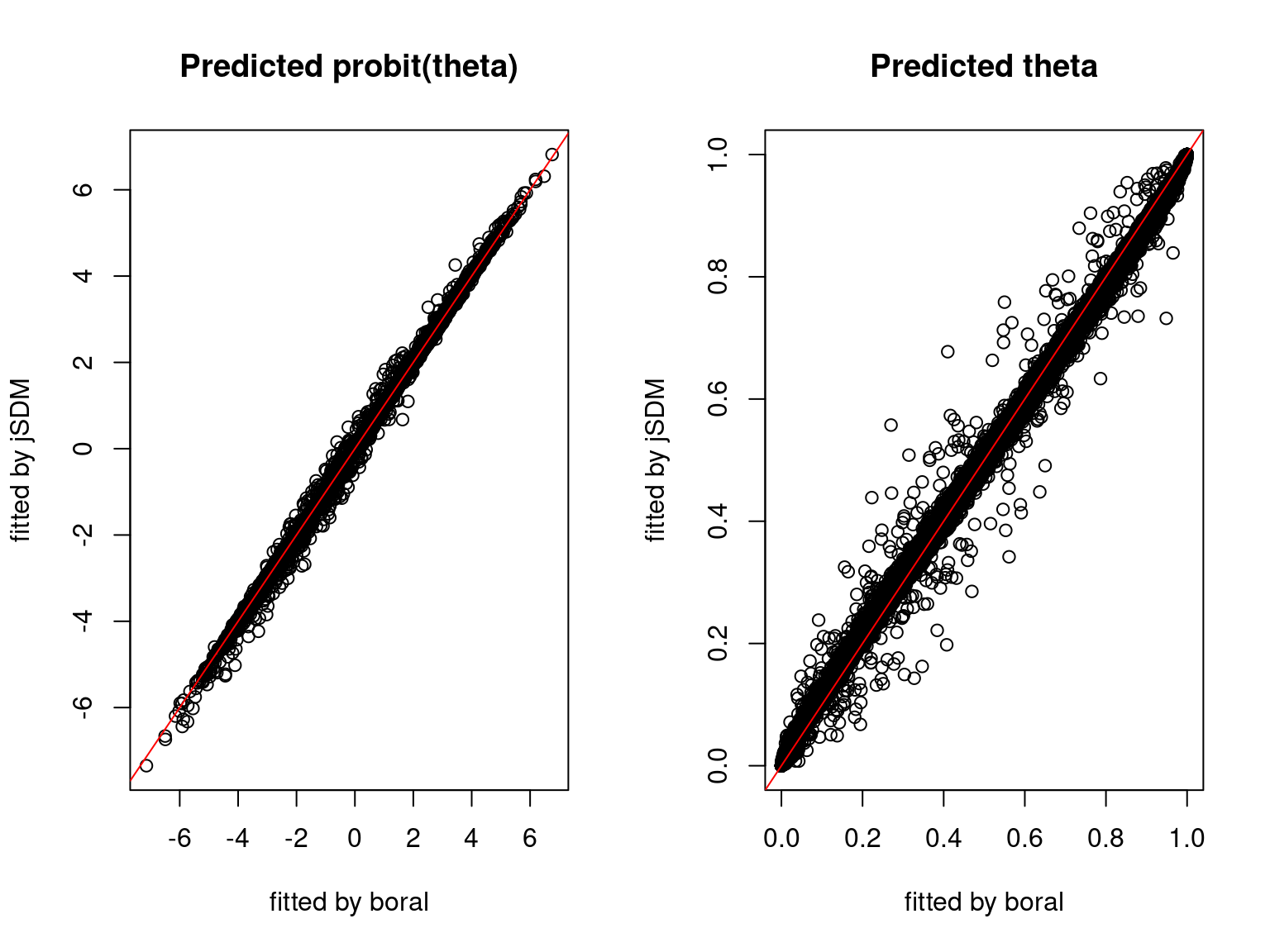
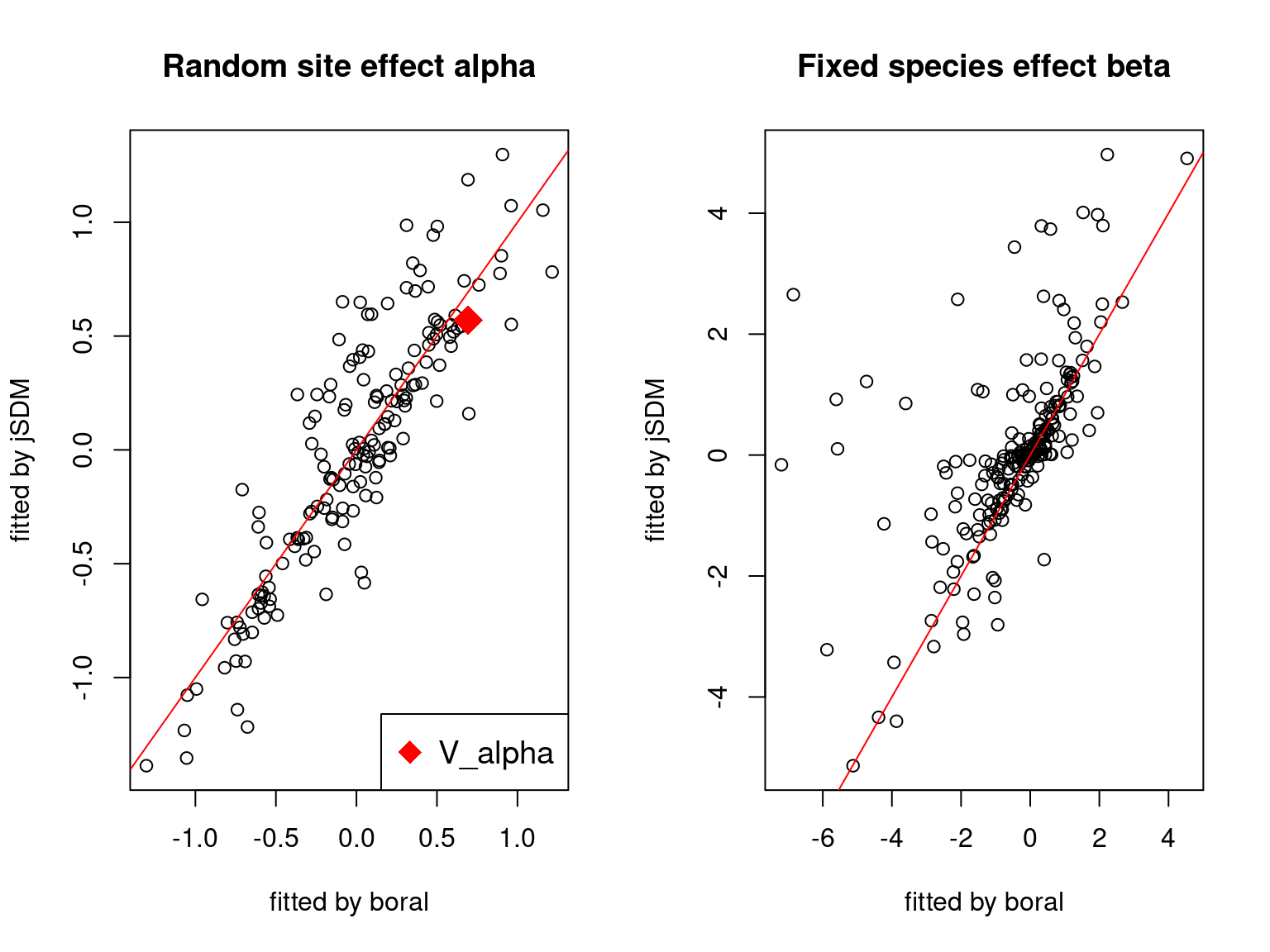
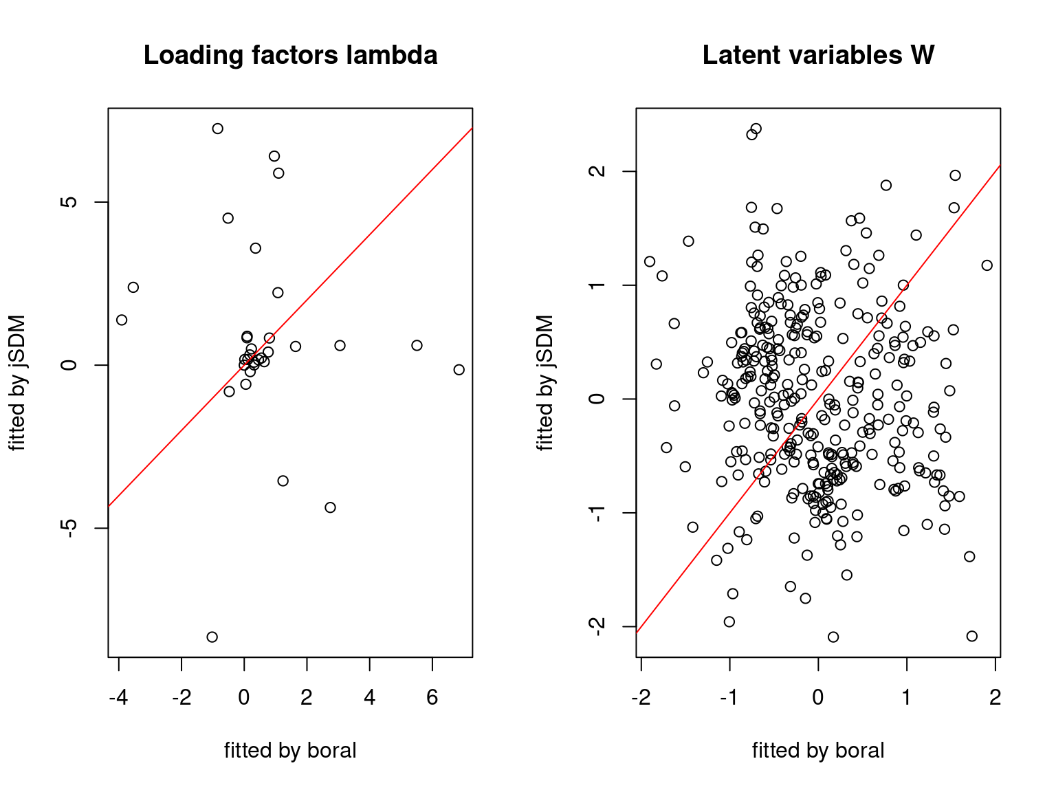
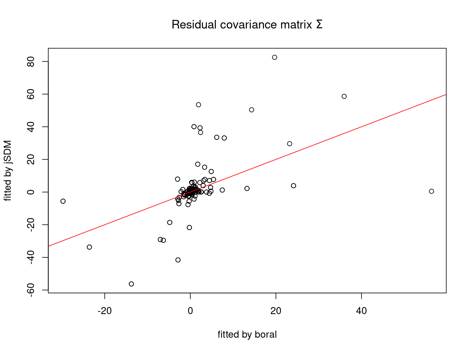
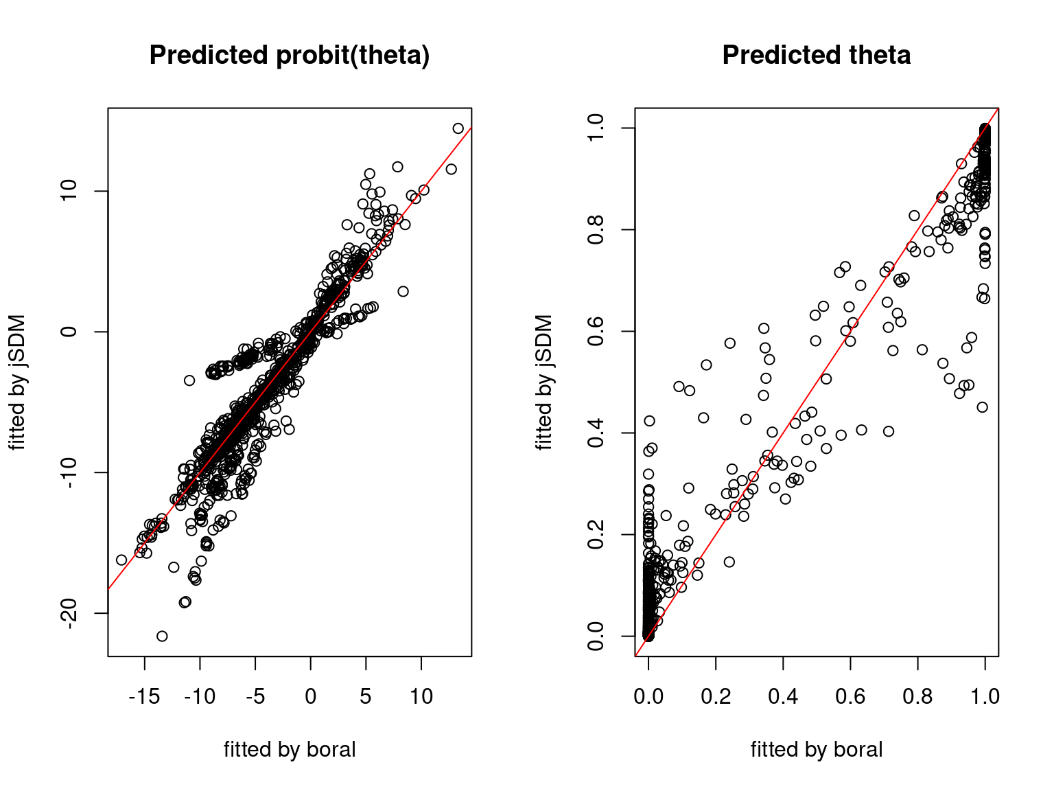
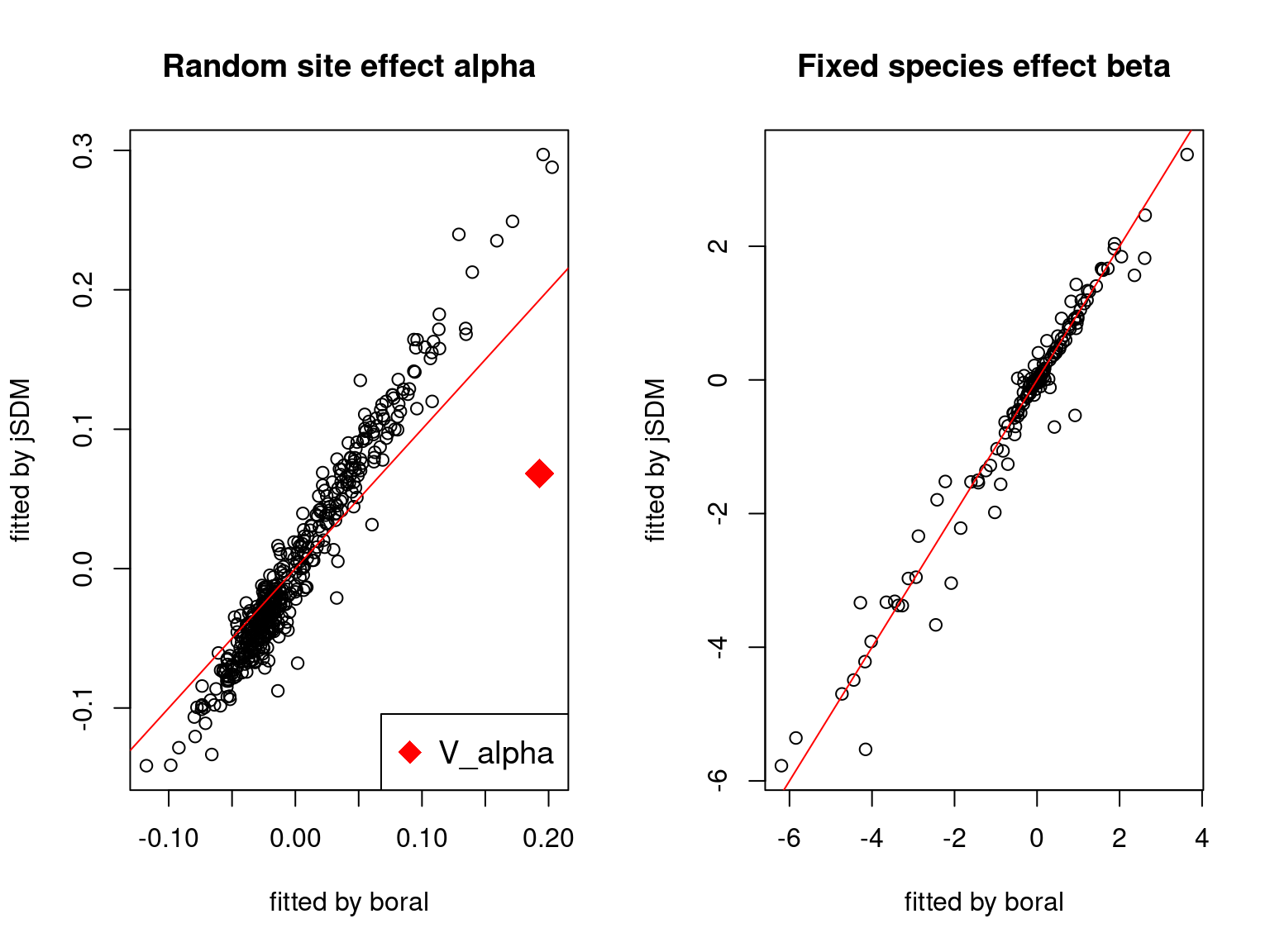
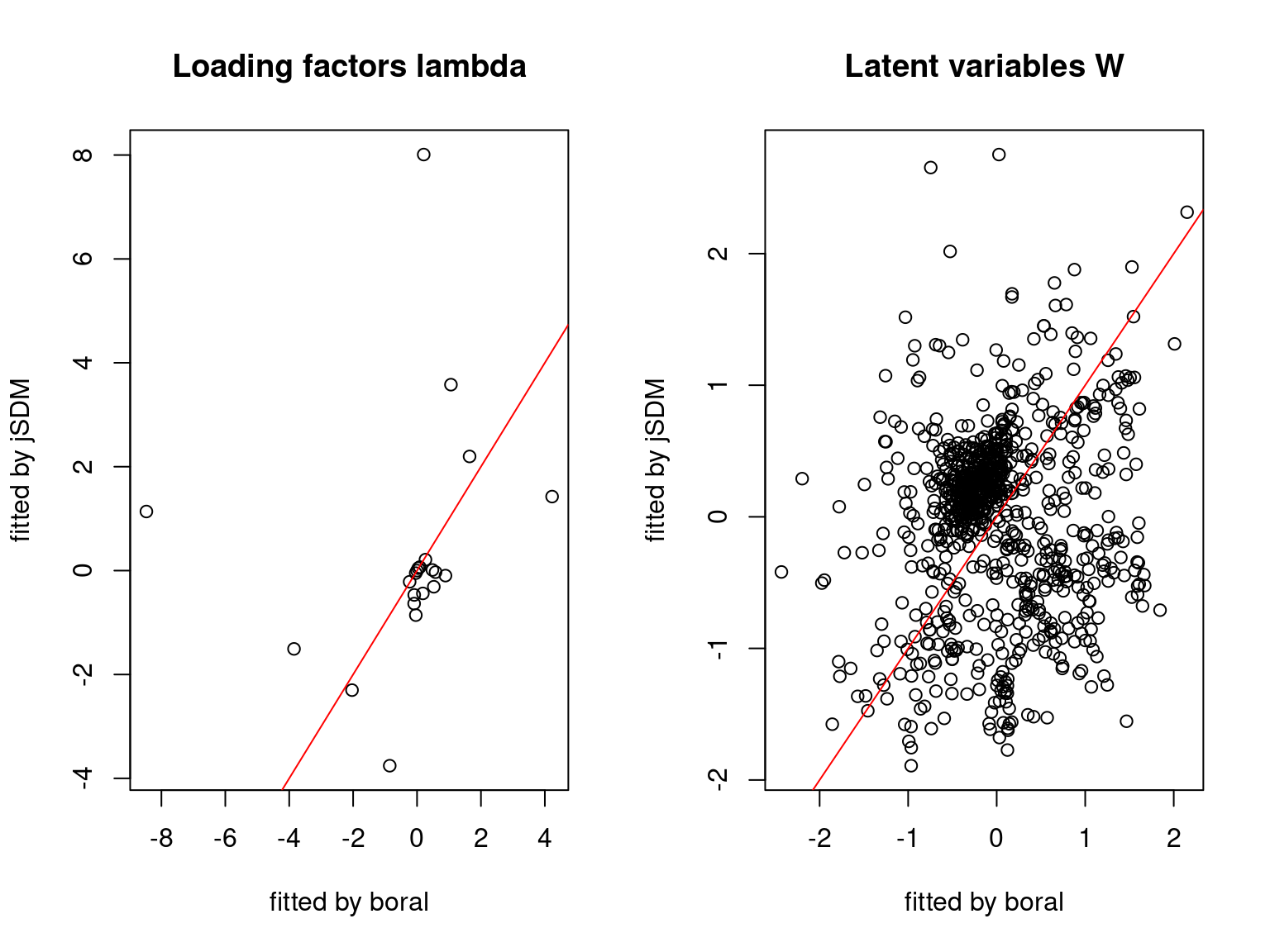
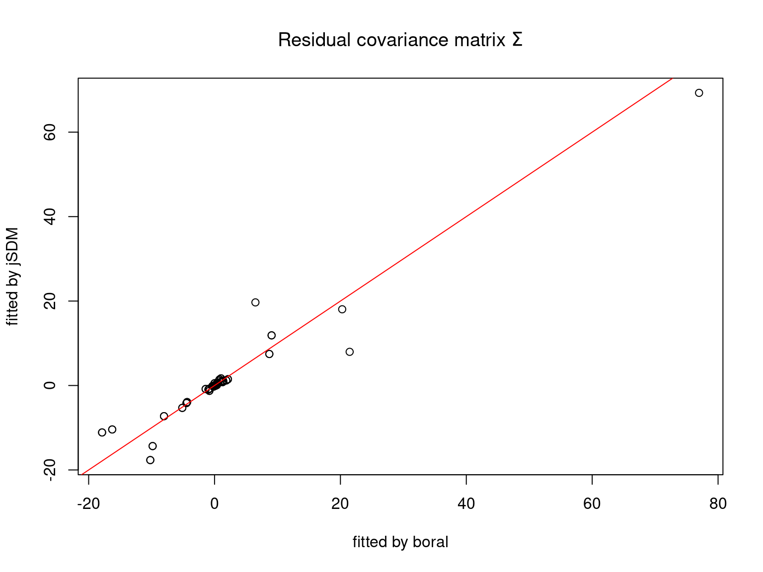
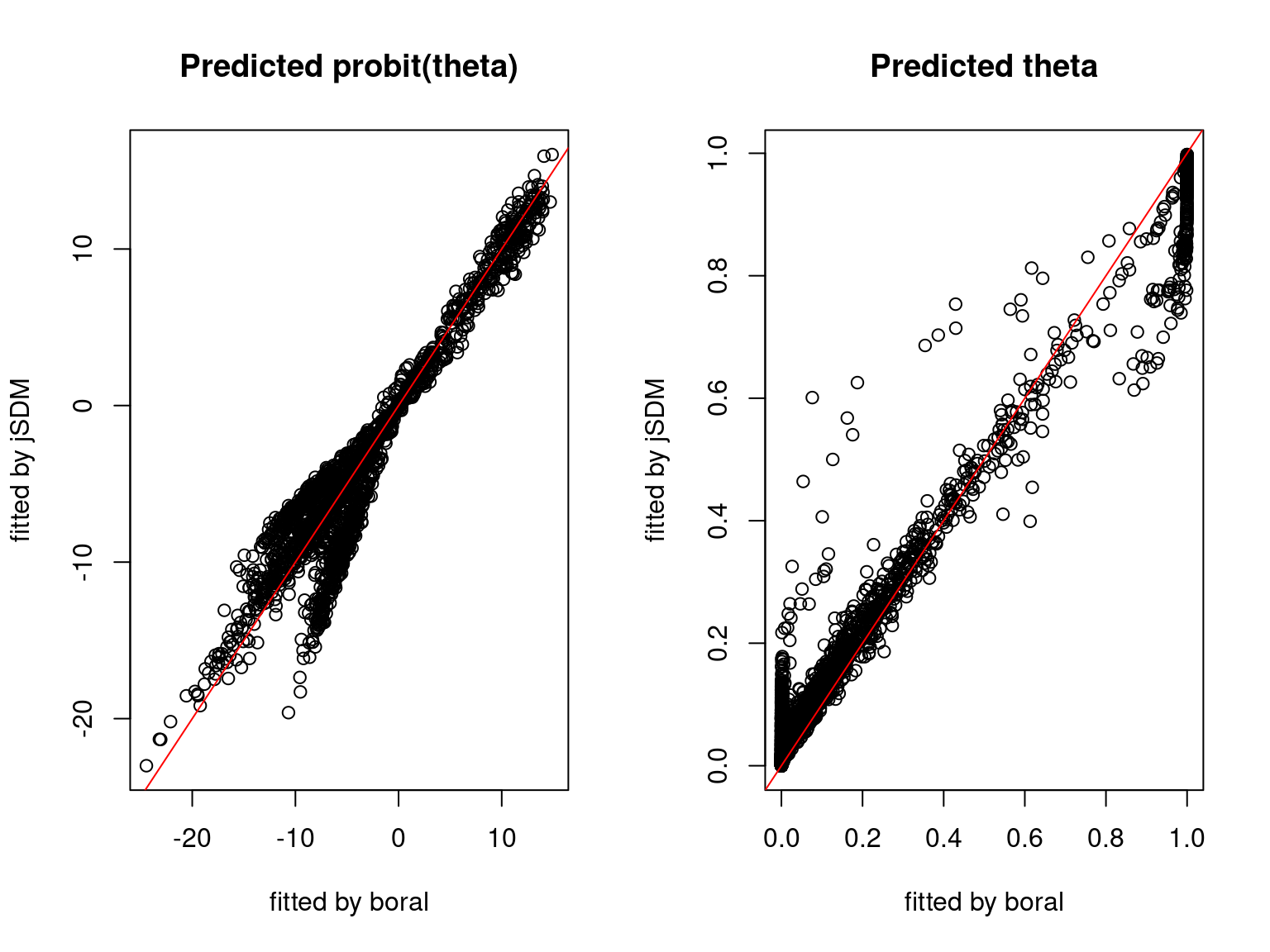
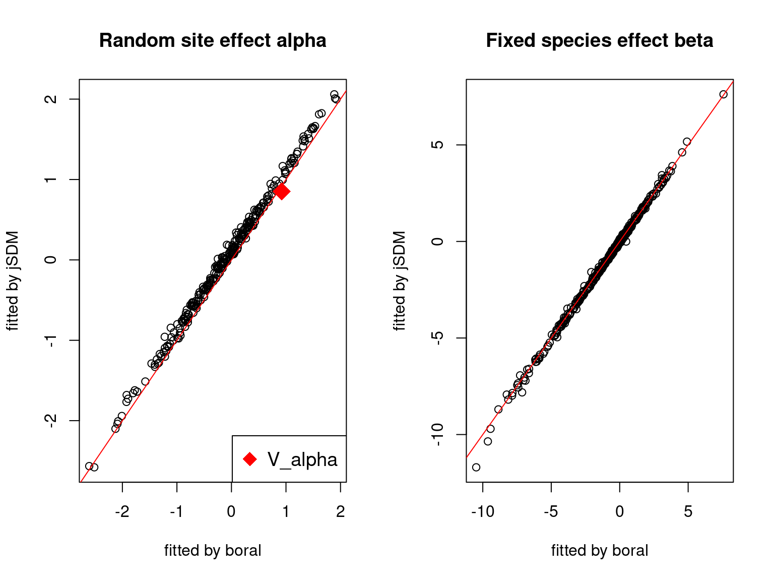
We plot the parameters estimated with jSDM against those estimated with boral to compare the results obtained with both packages.
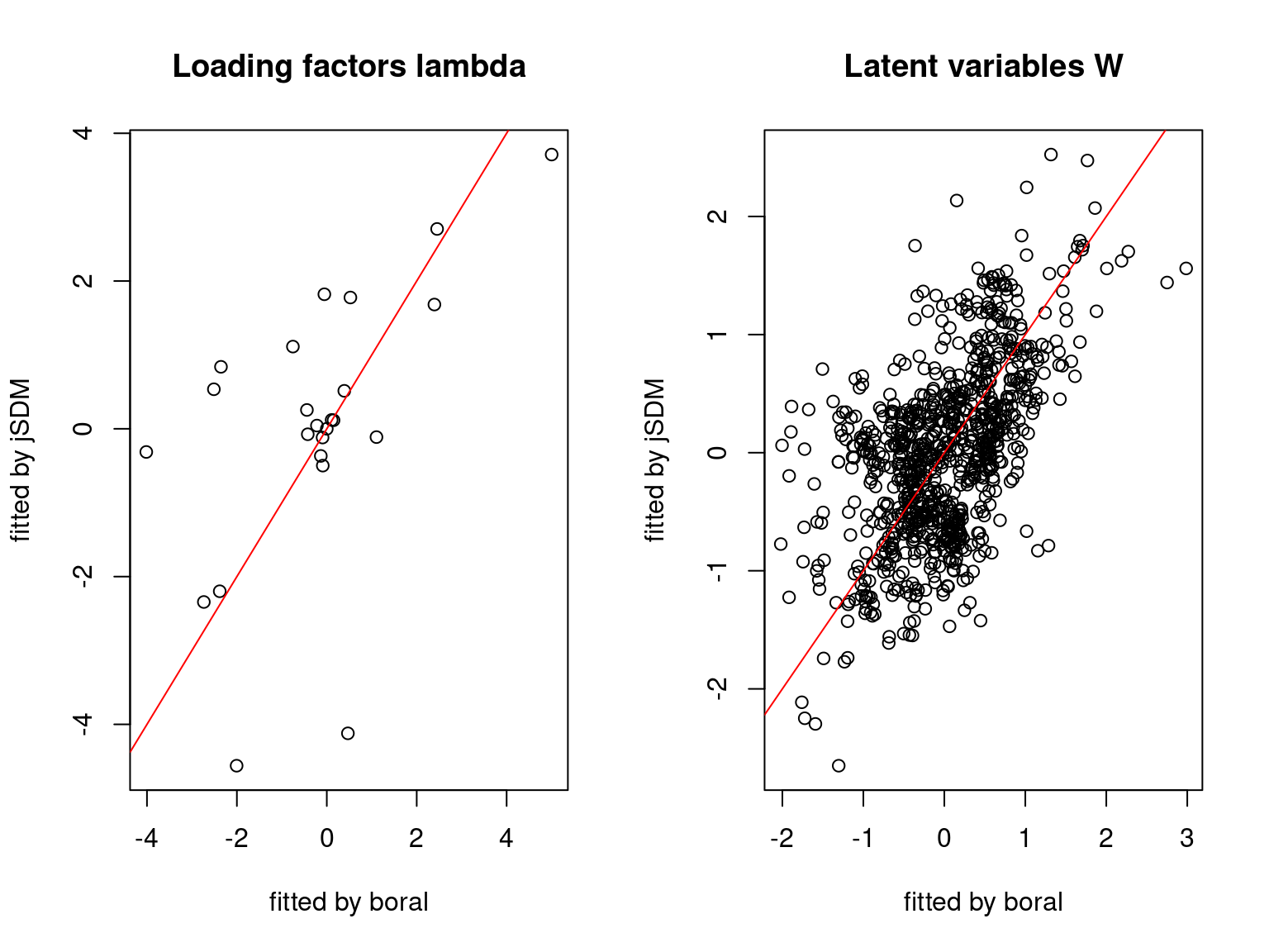
5.3.6 Birds dataset
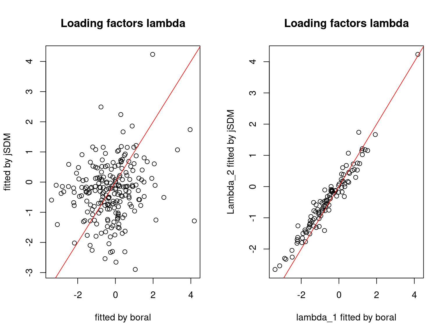
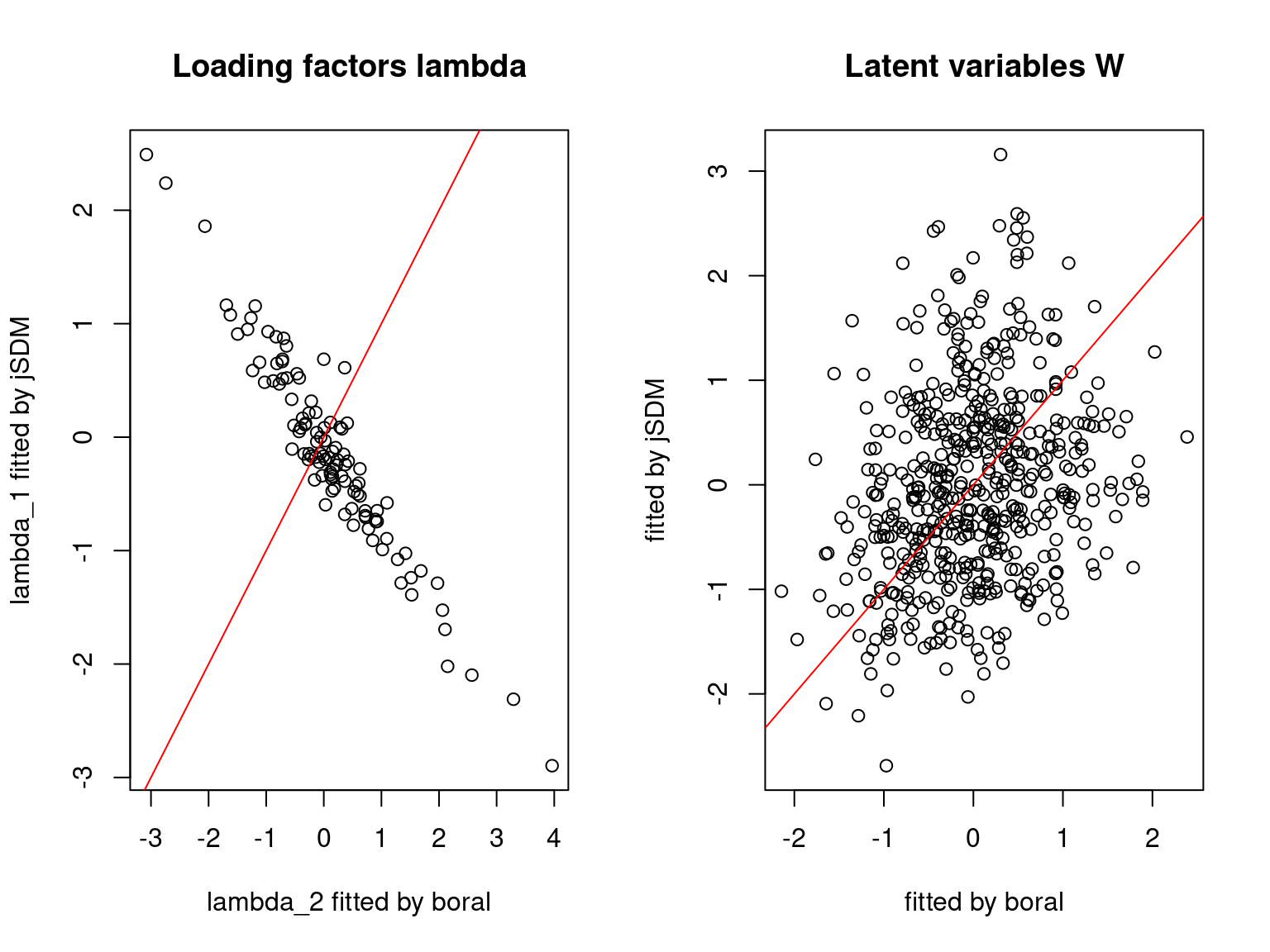
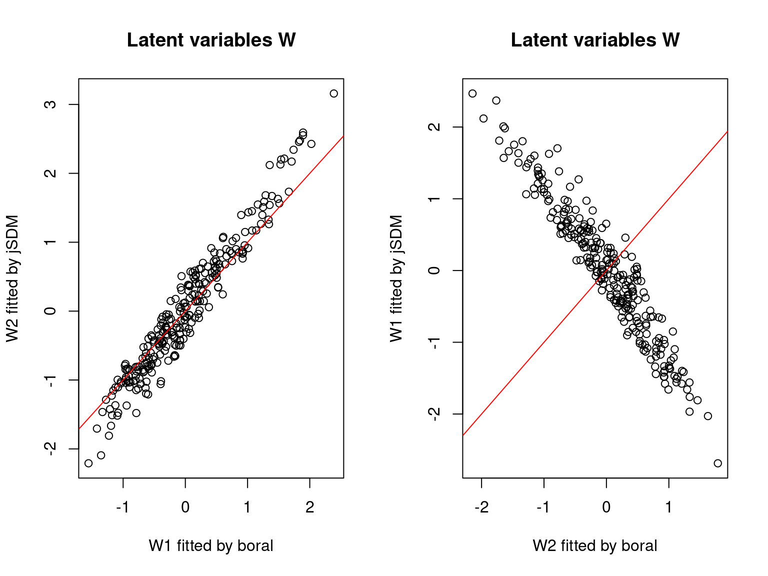
We can see an inversion of the order and signs of the latent axes estimated between jSDM and boral, indeed the first latent axis fitted with jSDM \(W_1\) corresponds to the second axis \(W_2\) in the results of boral, with opposite signs. Nevertheless, the presence probabilities and residual correlations predicted by the two packages are very close.
5.3.7 Mites dataset
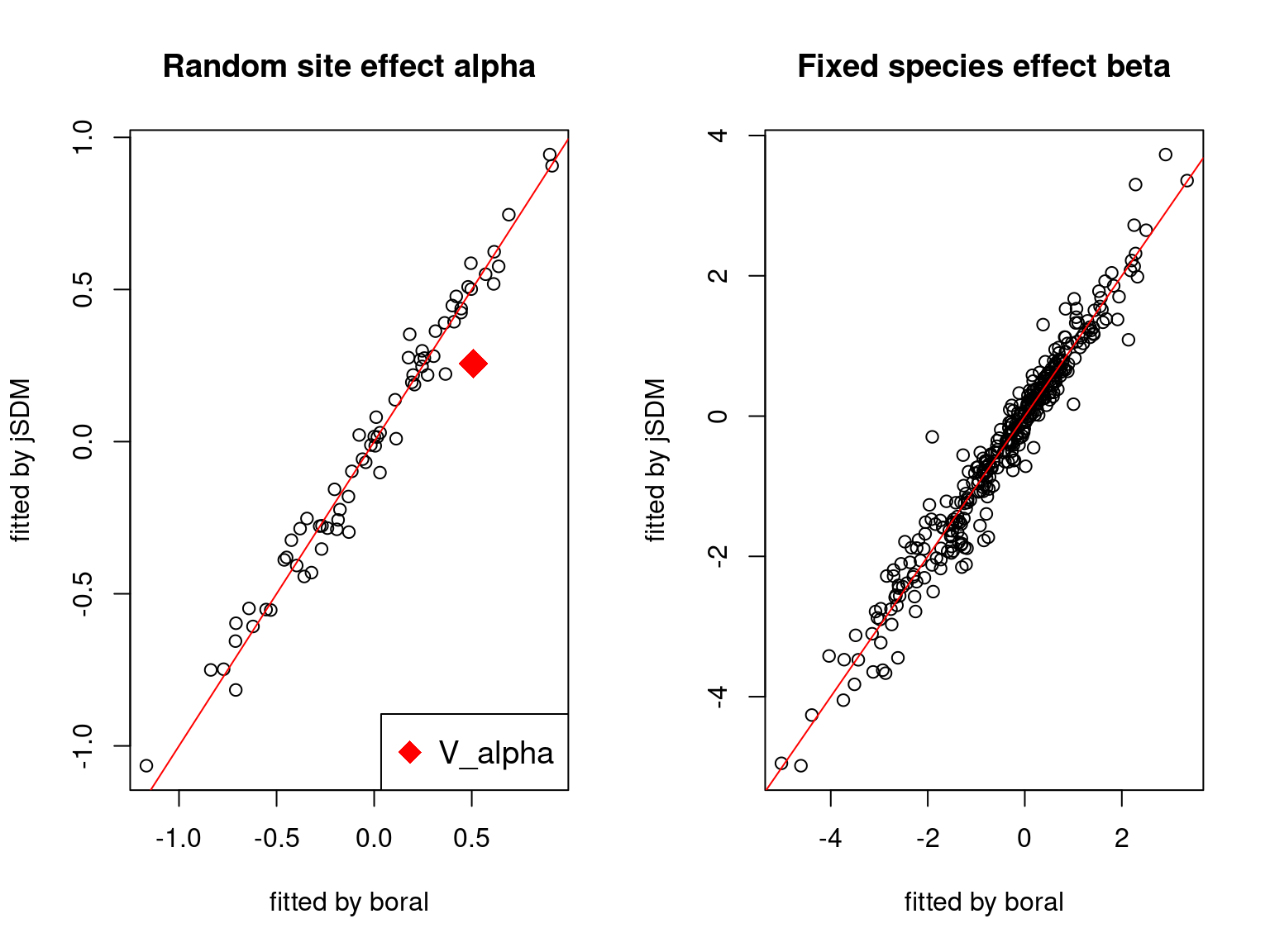
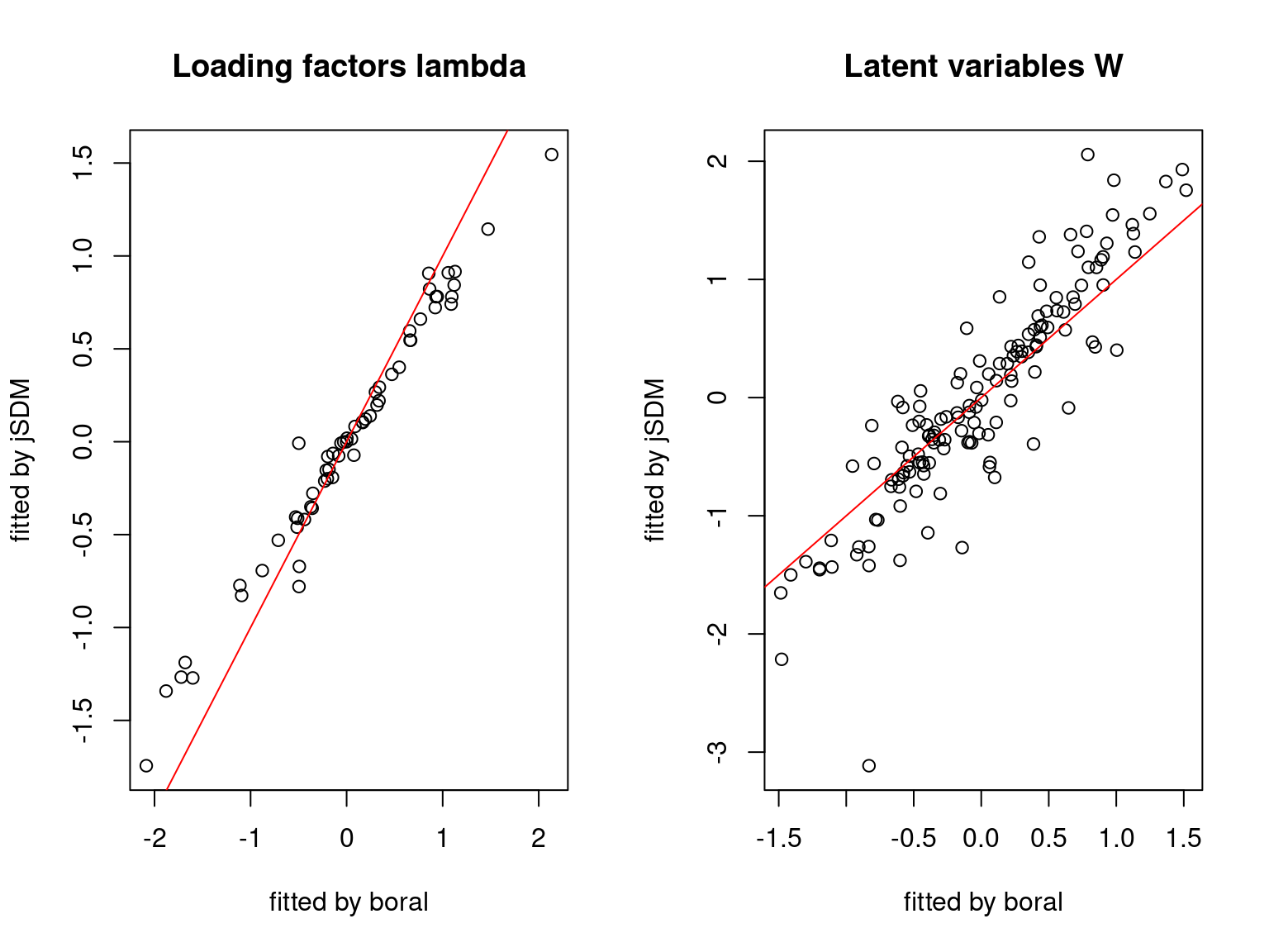
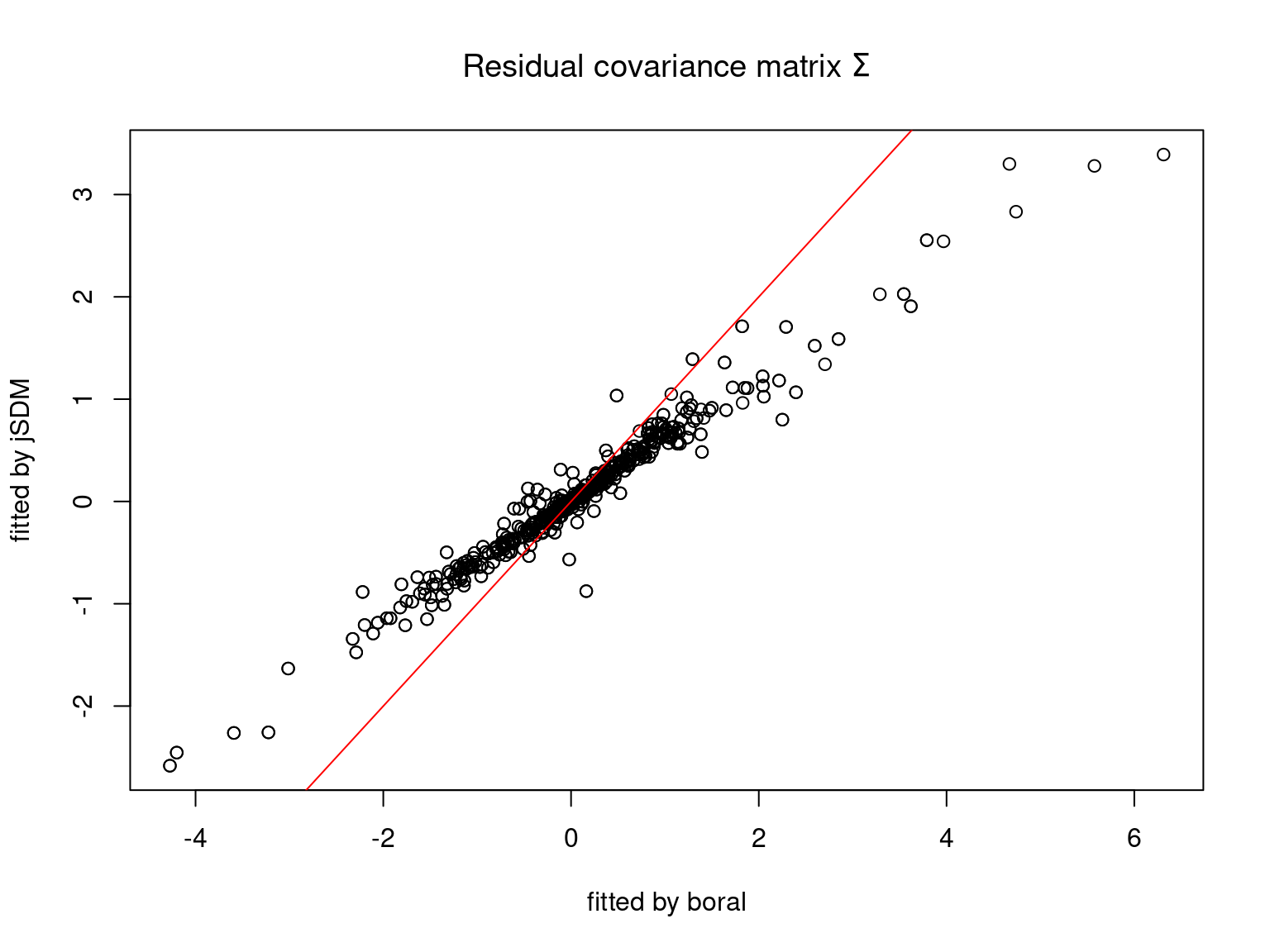
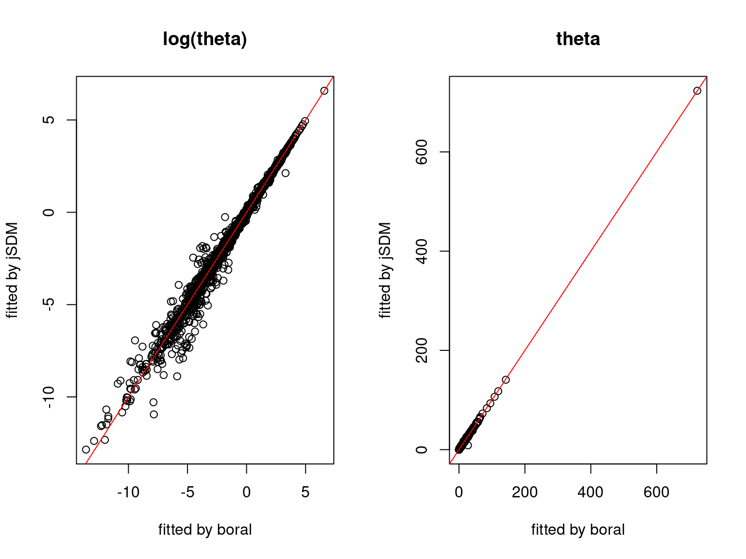
On the figures above, the parameters estimated with jSDM are close to those obtained with boral if the points are near the red line representing the identity function (\(y=x\)).