Get started with jSDM

1 jSDM package

jSDM is an R package for fitting joint species distribution models (JSDM) in a hierarchical Bayesian framework.

The Gibbs sampler is written in C++. It uses Rcpp, Armadillo and GSL to maximize computation efficiency.

Package:	jSDM
Type:	Package
Version:	0.2.1
Date:	2019-01-11
License:	GPL-3
LazyLoad:	yes

The package includes the following functions to fit various species distribution models :

function	data type	data format
jSDM_binomial_logit()	presence-absence	wide
jSDM_binomial_probit()	presence-absence	wide
jSDM_binomial_probit_sp_constrained()	presence-absence	wide
jSDM_binomial_probit_long_format()	presence-absence	long
jSDM_poisson_log()	abundance	wide
jSDM_gaussian()	continuous	wide

• jSDM_binomial_probit() :

  Ecological process:

  \[y_{ij} \sim \mathcal{B}ernoulli(\theta_{ij}),\] where

  conditions	model specification
  if n_latent=0 and site_effect="none"	probit\((\theta_{ij}) = \beta_{0j} + X_i \beta_j\)
  if n_latent>0 and site_effect="none"	probit\((\theta_{ij}) = \beta_{0j} + X_i \beta_j + W_i \lambda_j\)
  if n_latent=0 and site_effect="random"	probit\((\theta_{ij}) = \beta_{0j} + X_i \beta_j + \alpha_i\) and \(\alpha_i \sim \mathcal{N}(0,V_\alpha)\)
  if n_latent>0 and site_effect="fixed"	probit\((\theta_{ij}) = \beta_{0j} + X_i \beta_j + W_i \lambda_j + \alpha_i\)
  if n_latent=0 and site_effect="fixed"	probit\((\theta_{ij}) = \beta_{0j} + X_i \beta_j + \alpha_i\)
  if n_latent>0 and site_effect="random"	probit\((\theta_{ij}) = \beta_{0j} + X_i \beta_j + W_i \lambda_j + \alpha_i\) and \(\alpha_i \sim \mathcal{N}(0,V_\alpha)\)

• jSDM_binomial_probit_sp_constrained() :

  This function allows to fit the same models than the function jSDM_binomial_probit except for models not including latent variables, indeed n_latent must be greater than zero in this function.
  At first, the function fit a JSDM with the constrained species arbitrarily chosen as the first ones in the presence-absence data-set.
  Then, the function evaluates the convergence of MCMC \(\lambda\) chains using the Gelman-Rubin convergence diagnostic (Gelman & Rubin 1992) (\(\hat{R}\)). It identifies the species (\(\hat{j}_l\)) having the higher \(\hat{R}\) for \(\lambda_{\hat{j}_l}\). These species drive the structure of the latent axis \(l\). The \(\lambda\) corresponding to this species are constrained to be positive and placed on the diagonal of the \(\Lambda\) matrix for fitting a second model.
  This usually improves the convergence of the latent variables and factor loadings. The function returns the parameter posterior distributions for this second model.

• jSDM_binomial_logit() :

  Ecological process :

  \[y_{ij} \sim \mathcal{B}inomial(\theta_{ij},t_i),\] where

  conditions	model specification
  if n_latent=0 and site_effect="none"	logit\((\theta_{ij}) = \beta_{0j} + X_i \beta_j\)
  if n_latent>0 and site_effect="none"	logit\((\theta_{ij}) = \beta_{0j} + X_i \beta_j + W_i \lambda_j\)
  if n_latent=0 and site_effect="fixed"	logit\((\theta_{ij}) = \beta_{0j} + X_i \beta_j + \alpha_i\)
  if n_latent>0 and site_effect="fixed"	logit\((\theta_{ij}) = \beta_{0j} + X_i \beta_j + W_i \lambda_j + \alpha_i\)
  if n_latent=0 and site_effect="random"	logit\((\theta_{ij}) = \beta_{0j} + X_i \beta_j + \alpha_i\) and \(\alpha_i \sim \mathcal{N}(0,V_{\alpha})\)
  if n_latent>0 and site_effect="random"	logit\((\theta_{ij}) = \beta_{0j} + X_i \beta_j + W_i \lambda_j + \alpha_i\) and \(\alpha_i \sim \mathcal{N}(0,V_\alpha)\)

• jSDM_poisson_log() :

  Ecological process :

  \[y_{ij} \sim \mathcal{P}oisson(\theta_{ij}),\]

  where

  conditions	model specification
  if n_latent=0 and site_effect="none"	log\((\theta_{ij}) = \beta_{0j} + X_i \beta_j\)
  if n_latent>0 and site_effect="none"	log\((\theta_{ij}) = \beta_{0j} + X_i \beta_j + W_i \lambda_j\)
  if n_latent=0 and site_effect="fixed"	log\((\theta_{ij}) = \beta_{0j} + X_i \beta_j + \alpha_i\)
  if n_latent>0 and site_effect="fixed"	log\((\theta_{ij}) = \beta_{0j} + X_i \beta_j + W_i \lambda_j + \alpha_i\)
  if n_latent=0 and site_effect="random"	log\((\theta_{ij}) = \beta_{0j} + X_i \beta_j + \alpha_i\) and \(\alpha_i \sim \mathcal{N}(0,V_\alpha)\)
  if n_latent>0 and site_effect="random"	log\((\theta_{ij}) = \beta_{0j} + X_i \beta_j + W_i \lambda_j + \alpha_i\) and \(\alpha_i \sim \mathcal{N}(0,V_\alpha)\)

• jSDM_binomial_probit_long_format() :

  Ecological process:

  \[y_{n} \sim \mathcal{B}ernoulli(\theta_n),\] such as \(species_n=j\) and \(site_n=i\), where

  conditions	model specification
  if n_latent=0 and site_effect="none"	probit\((\theta_n) = D_n \gamma + X_n \beta_j\)
  if n_latent>0 and site_effect="none"	probit\((\theta_n) = D_n \gamma + X_n \beta_j + W_i \lambda_j\)
  if n_latent=0 and site_effect="random"	probit\((\theta_n) = D_n \gamma + X_n \beta_j + \alpha_i\) and \(\alpha_i \sim \mathcal{N}(0,V_\alpha)\)
  if n_latent>0 and site_effect="fixed"	probit\((\theta_n) = D_n \gamma + X_n \beta_j + W_i \lambda_j + \alpha_i\)
  if n_latent=0 and site_effect="fixed"	probit\((\theta_n) = D_n \gamma + X_n \beta_j + \alpha_i\)
  if n_latent>0 and site_effect="random"	probit\((\theta_n) = D_n \gamma + X_n \beta_j + W_i \lambda_j + \alpha_i\) and \(\alpha_i \sim \mathcal{N}(0,V_\alpha)\)

• jSDM_gaussian() :

  Ecological process:

  \[y_{ij} \sim \mathcal{N}(\theta_{ij}, V),\] where

  conditions	model specification
  if n_latent=0 and site_effect="none"	\(\theta_{ij} = \beta_{0j} + X_i \beta_j\)
  if n_latent>0 and site_effect="none"	\(\theta_{ij} = \beta_{0j} + X_i \beta_j + W_i \lambda_j\)
  if n_latent=0 and site_effect="random"	\(\theta_{ij} = \beta_{0j} + X_i \beta_j + \alpha_i\) and \(\alpha_i \sim \mathcal{N}(0,V_\alpha)\)
  if n_latent>0 and site_effect="fixed"	\(\theta_{ij} = \beta_{0j} + X_i \beta_j + W_i \lambda_j + \alpha_i\)
  if n_latent=0 and site_effect="fixed"	\(\theta_{ij} = \beta_{0j} + X_i \beta_j + \alpha_i\)
  if n_latent>0 and site_effect="random"	\(\theta_{ij} = \beta_{0j} + X_i \beta_j + W_i \lambda_j + \alpha_i\) and \(\alpha_i \sim \mathcal{N}(0,V_\alpha)\)

  Joint Species distribution models (jSDM) are useful tools to explain or predict species range and abundance from various environmental factors and species correlations (Warton et al. 2015). jSDM is becoming an increasingly popular statistical method in conservation biology.

In this vignette, we illustrate the use of the jSDM R package which aims at providing user-friendly statistical functions using field observations (occurrence or abundance data) to fit jSDMs models.

Package’s functions are developed in a hierarchical Bayesian framework and use adaptive rejection Metropolis sampling algorithms or conjugate priors within Gibbs sampling to estimate model’s parameters. Using compiled C++ code for the Gibbs sampler reduce drastically the computation time. By making these new statistical tools available to the scientific community, we hope to democratize the use of more complex, but more realistic, statistical models for increasing knowledge in ecology and conserving biodiversity.

Directed Acyclic Graph (DAG)

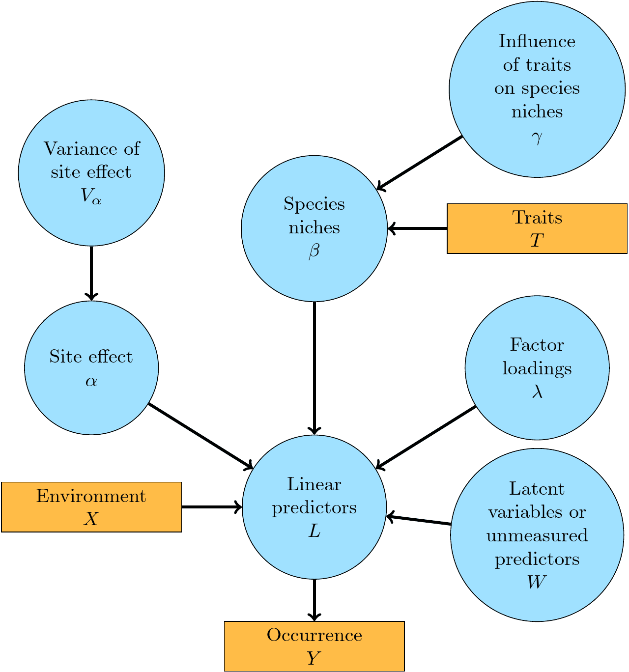
Figure 1.1: A graphical summary of the jSDM-package statistical framework. In this Directed Acyclic Graph (DAG), the orange boxes refer to data, the blue ellipses to parameters to be estimated, and the arrows to functional relationships described with the help of statistical distributions.

Model types available in jSDM R package are not limited to those described in this example. jSDM includes various model types for occurrence and abundance data, you can find more examples of use on the jSDM website.

2 Load librairies

We first load the jSDM library.

# Load libraries
library(jSDM)
#> ##
#> ## jSDM R package 
#> ## For joint species distribution models 
#> ## https://ecology.ghislainv.fr/jSDM 
#> ##

3 Bernoulli probit regression

Below, we show an example of the use of jSDM-package for fitting species distribution model to occurence data for 9 frog’s species.

3.1 Definition of the model

Referring to the models used in the articles Warton et al. (2015) and Albert & Siddhartha (1993), we define the following model :

\[ \mathrm{probit}(\theta_{ij}) =\alpha_i + \beta_{0j}+X_i.\beta_j+ W_i.\lambda_j \]

• Link function probit: \(\mathrm{probit}: q \rightarrow \Phi^{-1}(q)\) where \(\Phi\) correspond to the repartition function of the reduced centred normal distribution.

• Response variable: \(Y=(y_{ij})^{i=1,\ldots,nsite}_{j=1,\ldots,nsp}\) with:

\[y_{ij}=\begin{cases} 0 & \text{ if species $j$ is absent on the site $i$}\\ 1 & \text{ if species $j$ is present on the site $i$}. \end{cases}\]

• Latent variable \(z_{ij} = \alpha_i + \beta_{0j} + X_i.\beta_j + W_i.\lambda_j + \epsilon_{i,j}\), with \(\forall (i,j) \ \epsilon_{ij} \sim \mathcal{N}(0,1)\) and such that:

\[y_{ij}=\begin{cases} 1 & \text{if} \ z_{ij} > 0 \\ 0 & \text{otherwise.} \end{cases}\]

It can be easily shown that: \(y_{ij} \sim \mathcal{B}ernoulli(\theta_{ij})\).

• Latent variables: \(W_i=(W_i^1,\ldots,W_i^q)\) where \(q\) is the number of latent variables considered, which has to be fixed by the user (by default q=2). We assume that \(W_i \sim \mathcal{N}(0,I_q)\) and we define the associated coefficients: \(\lambda_j=(\lambda_j^1,\ldots, \lambda_j^q)'\). We use a prior distribution \(\mathcal{N}(0,1)\) for all lambdas not concerned by constraints to \(0\) on upper diagonal and to strictly positive values on diagonal.

• Explanatory variables: bioclimatic data about each site. \(X=(X_i)_{i=1,\ldots,nsite}\) with \(X_i=(x_i^1,\ldots,x_i^p)\in \mathbb{R}^p\) where \(p\) is the number of bioclimatic variables considered. The corresponding regression coefficients for each species \(j\) are noted : \(\beta_j=(\beta_j^1,\ldots,\beta_j^p)'\).

• \(\beta_{0j}\) correspond to the intercept for species \(j\) which is assume to be a fixed effect. We use a prior distribution \(\mathcal{N}(0,1)\) for all betas.

• \(\alpha_i\) represents the random effect of site \(i\) such as \(\alpha_i \sim \mathcal{N}(0,V_{\alpha})\) and we assumed that \(V_{\alpha} \sim \mathcal {IG}(\text{shape}=0.1, \text{rate}=0.1)\) as prior distribution by default.

3.2 Occurrence data-set

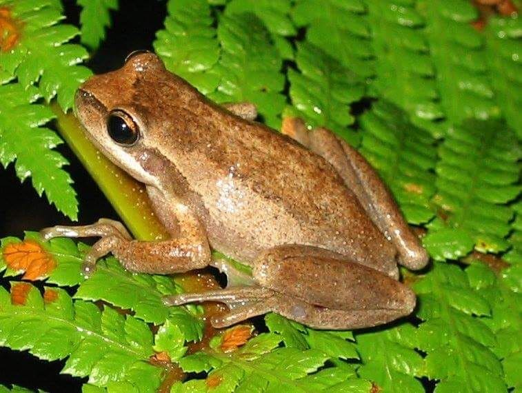
Figure 3.1: Litoria ewingii (Wilkinson et al. 2019).

This data-set is available in jSDM-package. It can be loaded with the data() command. The frogs dataset is in “wide” format: each line is a site and the occurrence data (from Species_1 to Species_9) are in columns. A site is characterized by its x-y geographical coordinates, one discrete covariate and two other continuous covariates.

# frogs data
data(frogs, package="jSDM")
head(frogs)
#>   Covariate_1 Covariate_2 Covariate_3 Species_1 Species_2 Species_3 Species_4
#> 1    3.870111           0    0.045334         1         0         0         0
#> 2    3.326950           1    0.115903         0         0         0         0
#> 3    2.856729           1    0.147034         0         0         0         0
#> 4    1.623249           1    0.124283         0         0         0         0
#> 5    4.629685           1    0.081655         0         0         0         0
#> 6    0.698970           1    0.107048         0         0         0         0
#>   Species_5 Species_6 Species_7 Species_8 Species_9        y        x
#> 1         0         0         0         0         0 66.41479 9.256424
#> 2         0         1         0         0         0 67.03841 9.025588
#> 3         0         1         0         0         0 67.03855 9.029416
#> 4         0         1         0         0         0 67.04200 9.029745
#> 5         0         1         0         0         0 67.04439 9.026514
#> 6         0         0         0         0         0 67.03894 9.023580

We rearrange the data in two data-sets: a first one for the presence-absence observations for each species (columns) at each site (rows), and a second one for the site characteristics.

We also normalize the continuous explanatory variables to facilitate MCMC convergence.

# data.obs
PA_frogs <- frogs[,4:12]

# Normalized continuous variables
Env_frogs <- cbind(scale(frogs[,1]),frogs[,2],scale(frogs[,3]))
colnames(Env_frogs) <- colnames(frogs[,1:3])

3.3 Parameter inference

We use the jSDM_binomial_probit() function to fit the jSDM (increase the number of iterations to achieve convergence).

mod_frogs_jSDM_probit <- jSDM_binomial_probit(
  # Chains
  burnin=1000, mcmc=1000, thin=1,
  # Response variable 
  presence_data = PA_frogs, 
  # Explanatory variables 
  site_formula = ~.,   
  site_data = Env_frogs,
  # Model specification 
  n_latent=2, site_effect="random",
  # Starting values
  alpha_start=0, beta_start=0,
  lambda_start=0, W_start=0,
  V_alpha=1, 
  # Priors
  shape_Valpha=0.1,
  rate_Valpha=0.1,
  mu_beta=0, V_beta=1,
  mu_lambda=0, V_lambda=1,
  # Various 
  seed=1234, verbose=1)
#> 
#> Running the Gibbs sampler. It may be long, please keep cool :)
#> 
#> **********:10.0% 
#> **********:20.0% 
#> **********:30.0% 
#> **********:40.0% 
#> **********:50.0% 
#> **********:60.0% 
#> **********:70.0% 
#> **********:80.0% 
#> **********:90.0% 
#> **********:100.0%

3.4 Analysis of the results

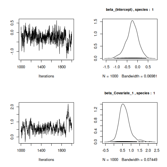
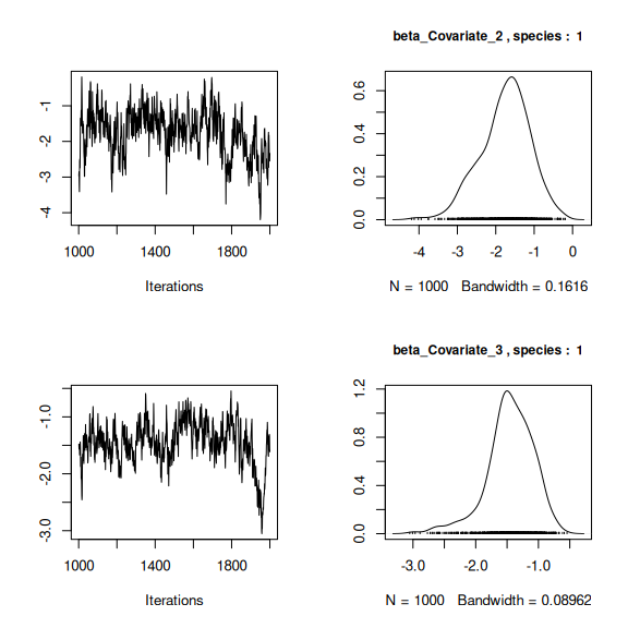
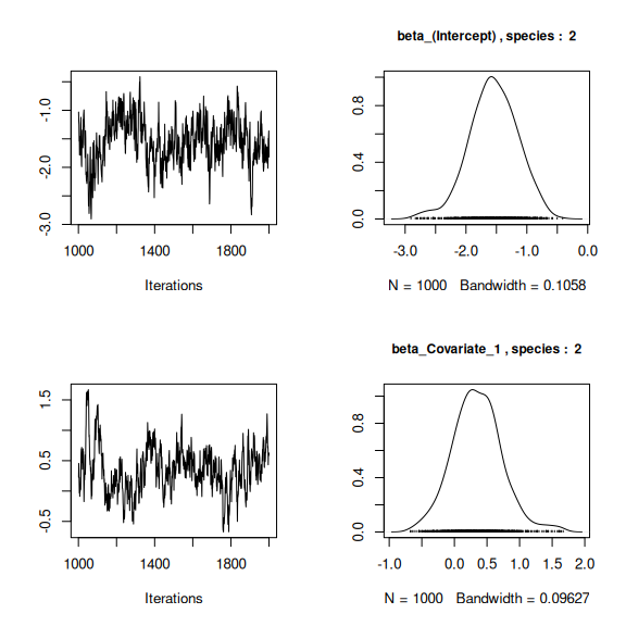
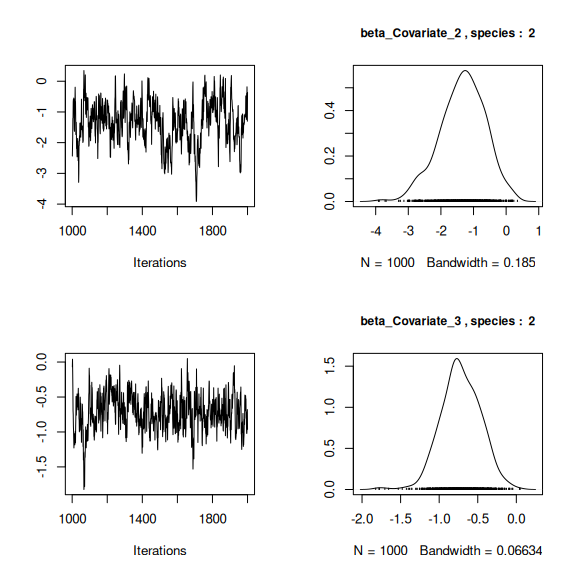
We visually evaluate the convergence of MCMCs by representing the trace and density a posteriori of some estimated parameters.

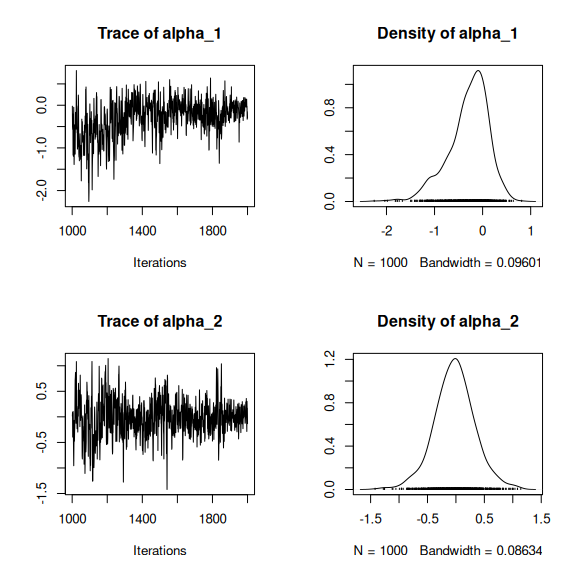
np <- nrow(mod_frogs_jSDM_probit$model_spec$beta_start)

## beta_j of the first two species
par(mfrow=c(2,2))
for (j in 1:2) {
  for (p in 1:np) {
    coda::traceplot(coda::as.mcmc(mod_frogs_jSDM_probit$mcmc.sp[[j]][,p]))
    coda::densplot(coda::as.mcmc(mod_frogs_jSDM_probit$mcmc.sp[[j]][,p]), 
                   main = paste(colnames(mod_frogs_jSDM_probit$mcmc.sp[[j]])[p],
                                ", species : ",j), cex.main=0.9)
  }
}

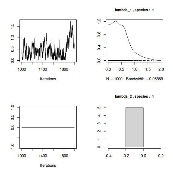
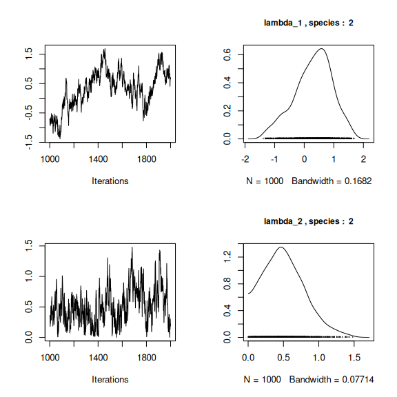
## lambda_j of the first two species
n_latent <- mod_frogs_jSDM_probit$model_spec$n_latent
par(mfrow=c(2,2))
for (j in 1:2) {
  for (l in 1:n_latent) {
    coda::traceplot(coda::as.mcmc(mod_frogs_jSDM_probit$mcmc.sp[[j]][,np+l]))
    coda::densplot(coda::as.mcmc(mod_frogs_jSDM_probit$mcmc.sp[[j]][,np+l]), 
                   main = paste(colnames(mod_frogs_jSDM_probit$mcmc.sp[[j]])
                                [np+l],", species : ",j), cex.main=0.9)
  }
}

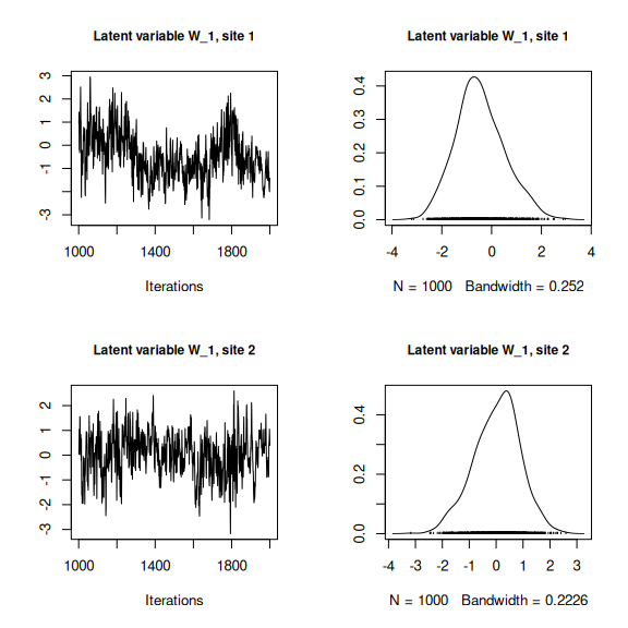
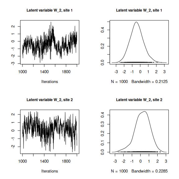
## Latent variables W_i for the first two sites
par(mfrow=c(2,2))
for (l in 1:n_latent) {
  for (i in 1:2) {
  coda::traceplot(mod_frogs_jSDM_probit$mcmc.latent[[paste0("lv_",l)]][,i],
                  main = paste0("Latent variable W_", l, ", site ", i),
                  cex.main=0.9)
  coda::densplot(mod_frogs_jSDM_probit$mcmc.latent[[paste0("lv_",l)]][,i],
                 main = paste0("Latent variable W_", l, ", site ", i),
                 cex.main=0.9)
  }
}

## alpha_i of the first two sites
plot(coda::as.mcmc(mod_frogs_jSDM_probit$mcmc.alpha[,1:2]))

## V_alpha
par(mfrow=c(2,2))
coda::traceplot(mod_frogs_jSDM_probit$mcmc.V_alpha)
coda::densplot(mod_frogs_jSDM_probit$mcmc.V_alpha)
## Deviance
coda::traceplot(mod_frogs_jSDM_probit$mcmc.Deviance)
coda::densplot(mod_frogs_jSDM_probit$mcmc.Deviance)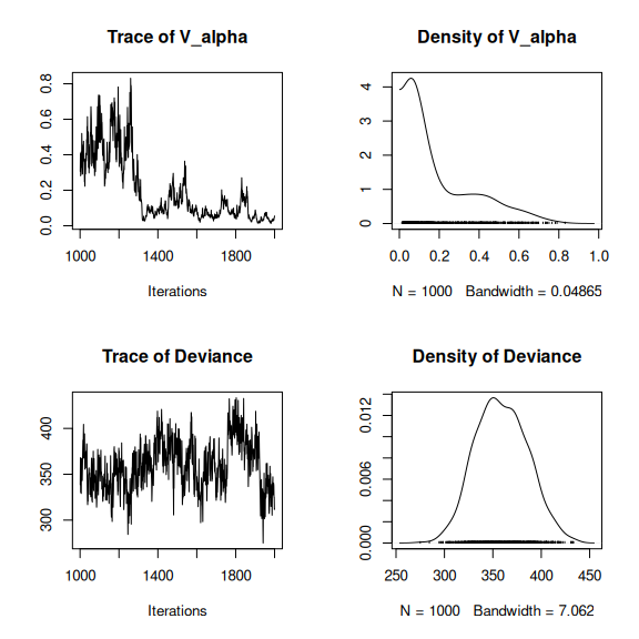

## probit_theta
par (mfrow=c(1,2))
hist(mod_frogs_jSDM_probit$probit_theta_latent,
     main = "Predicted probit theta",
     xlab ="predicted probit theta")
hist(mod_frogs_jSDM_probit$theta_latent,
     main = "Predicted theta", 
     xlab ="predicted theta")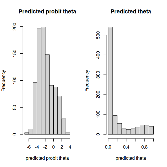

Overall, the traces and the densities of the parameters indicate the convergence of the algorithm. Indeed, we observe on the traces that the values oscillate around averages without showing an upward or downward trend and we see that the densities are quite smooth and for the most part of Gaussian form.

3.5 Matrice of correlations

After fitting the jSDM with latent variables, the full species residual correlation matrix \(R=(R_{ij})^{i=1,\ldots, n_{species}}_{j=1,\ldots, n_{species}}\) can be derived from the covariance in the latent variables such as : \[\Sigma_{ij} = \lambda_i^T .\lambda_j \], then we compute correlations from covariances : \[R_{i,j} = \frac{\Sigma_{ij}}{\sqrt{\Sigma _{ii}\Sigma _{jj}}}\].

We use the function plot_residual_cor() to compute and display the residual correlation matrix between species :

plot_residual_cor(mod_frogs_jSDM_probit)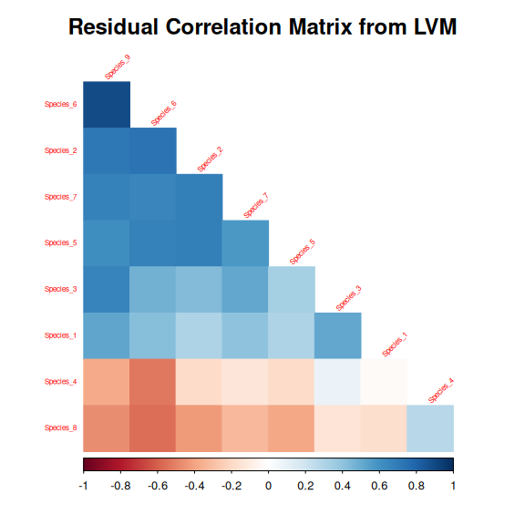

3.6 Predictions

We use the predict.jSDM() S3 method on the mod_frogs_jSDM_probit object of class jSDM to compute the mean (or expectation) of the posterior distributions obtained and get the expected values of model’s parameters.

# Sites and species concerned by predictions :
## 50 sites among the 104
Id_sites <- sample.int(nrow(PA_frogs), 50)
## All species 
Id_species <- colnames(PA_frogs)
# Simulate new observations of covariates on those sites 
simdata <- matrix(nrow=50, ncol = ncol(mod_frogs_jSDM_probit$model_spec$site_data))
colnames(simdata) <- colnames(mod_frogs_jSDM_probit$model_spec$site_data)
rownames(simdata) <- Id_sites
simdata <- as.data.frame(simdata)
simdata$Covariate_1 <- rnorm(50)
simdata$Covariate_3 <- rnorm(50)
simdata$Covariate_2 <- rbinom(50,1,0.5)

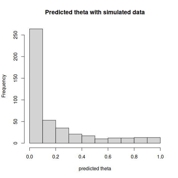
# Predictions 
theta_pred <- predict(mod_frogs_jSDM_probit, newdata=simdata, Id_species=Id_species,
                      Id_sites=Id_sites, type="mean")
hist(theta_pred, main="Predicted theta with simulated data", xlab="predicted theta")

References

Albert, J.H. & Siddhartha, C. (1993) Bayesian analysis of binary and polychotomous response data. Journal of the American Statistical Association, 88, 669–679.

Gelman, A. & Rubin, D.B. (1992) Inference from Iterative Simulation Using Multiple Sequences. Statistical Science, 7, 457–472.

Warton, D.I., Blanchet, F.G., O’Hara, R.B., Ovaskainen, O., Taskinen, S., Walker, S.C. & Hui, F.K.C. (2015) So many variables: Joint modeling in community ecology. Trends in Ecology & Evolution, 30, 766–779.

Wilkinson, D.P., Golding, N., Guillera-Arroita, G., Tingley, R. & McCarthy, M.A. (2019) A comparison of joint species distribution models for presence-absence data. Methods in Ecology and Evolution, 10, 198–211.