Plot the residual correlation matrix from a latent variable model (LVM).

Plot the posterior mean estimator of residual correlation matrix reordered by first principal component using corrplot function from the package of the same name.

plot_residual_cor(
  mod,
  prob = NULL,
  main = "Residual Correlation Matrix from LVM",
  cex.main = 1.5,
  diag = FALSE,
  type = "lower",
  method = "color",
  mar = c(1, 1, 3, 1),
  tl.srt = 45,
  tl.cex = 0.5,
  ...
)

Arguments

mod: An object of class "jSDM".
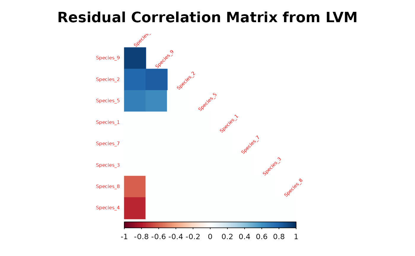
prob: A numeric scalar in the interval \((0,1)\) giving the target probability coverage of the intervals, by which to determine whether the correlations are "significant". If prob=0.95 is specified only significant correlations, whose \(95\%\) HPD interval does not contain zero, are represented. Defaults to prob=NULL to represent all correlations significant or not.
main: Character, title of the graph.
cex.main: Numeric, title's size.
diag: Logical, whether display the correlation coefficients on the principal diagonal.
type: Character, "full" (default), "upper" or "lower", display full matrix, lower triangular or upper triangular matrix.
method: Character, the visualization method of correlation matrix to be used. Currently, it supports seven methods, named "circle" (default), "square", "ellipse", "number", "pie", "shade" and "color".
mar: See par
tl.srt: Numeric, for text label string rotation in degrees, see text.
tl.cex: Numeric, for the size of text label (variable names).
...: Further arguments passed to corrplot function

Value

No return value. Displays a reordered correlation matrix.

References

Taiyun Wei and Viliam Simko (2017). R package "corrplot": Visualization of a Correlation Matrix (Version 0.84)

Warton, D. I.; Blanchet, F. G.; O'Hara, R. B.; O'Hara, R. B.; Ovaskainen, O.; Taskinen, S.; Walker, S. C. and Hui, F. K. C. (2015) So Many Variables: Joint Modeling in Community Ecology. Trends in Ecology & Evolution, 30, 766-779.

Author

Ghislain Vieilledent <ghislain.vieilledent@cirad.fr>

Jeanne Clément <jeanne.clement16@laposte.net>

Examples

library(jSDM)
# frogs data
data(frogs, package="jSDM")
# Arranging data
PA_frogs <- frogs[,4:12]
# Normalized continuous variables
 Env_frogs <- cbind(scale(frogs[,1]),frogs[,2],scale(frogs[,3]))
 colnames(Env_frogs) <- colnames(frogs[,1:3])
# Parameter inference
# Increase the number of iterations to reach MCMC convergence
mod<-jSDM_binomial_probit(# Response variable
                           presence_data = PA_frogs,
                           # Explanatory variables
                           site_formula = ~.,
                           site_data = Env_frogs,
                           n_latent=2,
                           site_effect="random",
                           # Chains
                           burnin=100,
                           mcmc=100,
                           thin=1,
                           # Starting values
                           alpha_start=0,
                           beta_start=0,
                           lambda_start=0,
                           W_start=0,
                           V_alpha=1,
                           # Priors
                           shape=0.1, rate=0.1,
                           mu_beta=0, V_beta=1,
                           mu_lambda=0, V_lambda=1,
                           # Various
                           seed=1234, verbose=1)
#> 
#> Running the Gibbs sampler. It may be long, please keep cool :)
#> 
#> **********:10.0% 
#> **********:20.0% 
#> **********:30.0% 
#> **********:40.0% 
#> **********:50.0% 
#> **********:60.0% 
#> **********:70.0% 
#> **********:80.0% 
#> **********:90.0% 
#> **********:100.0% 
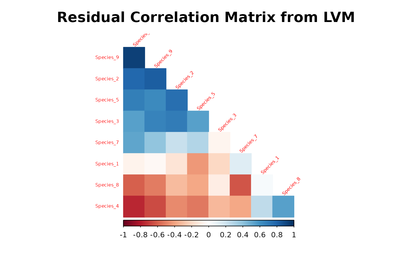
# Representation of residual correlation between species
plot_residual_cor(mod)

plot_residual_cor(mod, prob=0.95)