Binomial logistic regression

The jSDM_binomial_logit function performs a Binomial logistic regression in a Bayesian framework. The function calls a Gibbs sampler written in 'C++' code which uses an adaptive Metropolis algorithm to estimate the conditional posterior distribution of model's parameters.

jSDM_binomial_logit(
  burnin = 5000,
  mcmc = 10000,
  thin = 10,
  presence_data,
  site_formula,
  trait_data = NULL,
  trait_formula = NULL,
  site_data,
  trials = NULL,
  n_latent = 0,
  site_effect = "none",
  beta_start = 0,
  gamma_start = 0,
  lambda_start = 0,
  W_start = 0,
  alpha_start = 0,
  V_alpha = 1,
  shape_Valpha = 0.5,
  rate_Valpha = 5e-04,
  mu_beta = 0,
  V_beta = 10,
  mu_gamma = 0,
  V_gamma = 10,
  mu_lambda = 0,
  V_lambda = 10,
  ropt = 0.44,
  seed = 1234,
  verbose = 1
)

Arguments

burnin: The number of burnin iterations for the sampler.
mcmc: The number of Gibbs iterations for the sampler. Total number of Gibbs iterations is equal to burnin+mcmc. burnin+mcmc must be divisible by 10 and superior or equal to 100 so that the progress bar can be displayed.
thin: The thinning interval used in the simulation. The number of mcmc iterations must be divisible by this value.
presence_data: A matrix $n_{site} \times n_{species}$ indicating the number of successes (or presences) and the absence by a zero for each species at the studied sites.
site_formula: A one-sided formula of the form '~x1+...+xp' specifying the explanatory variables for the suitability process of the model, used to form the design matrix $X$ of size $n_{site} \times np$.
trait_data: A data frame containing the species traits which can be included as part of the model. Default to NULL to fit a model without species traits.
trait_formula: A one-sided formula of the form '~ t1 + ... + tk + x1:t1 + ... + xp:tk' specifying the interactions between the environmental variables and the species traits to be considered in the model, used to form the trait design matrix $Tr$ of size $n_{species} \times nt$ and to set to $0$ the $\gamma$ parameters corresponding to interactions not taken into account according to the formula. Default to NULL to fit a model with all possible interactions between species traits found in trait_data and environmental variables defined by site_formula.
site_data: A data frame containing the model's explanatory variables by site.
trials: A vector indicating the number of trials for each site. $n_i$ should be superior or equal to $y_{ij}$, the number of successes for observation $n$. If $n_i=0$, then $y_{ij}=0$. The default is one visit by site.
n_latent: An integer which specifies the number of latent variables to generate. Defaults to $0$.
site_effect: A string indicating whether row effects are included as fixed effects ("fixed"), as random effects ("random"), or not included ("none") in the model. If fixed effects, then for parameter identifiability the first row effect is set to zero, which analogous to acting as a reference level when dummy variables are used. If random effects, they are drawn from a normal distribution with mean zero and unknown variance, analogous to a random intercept in mixed models. Defaults to "none".
beta_start: Starting values for $\beta$ parameters of the suitability process for each species must be either a scalar or a $np \times n_{species}$ matrix. If beta_start takes a scalar value, then that value will serve for all of the $\beta$ parameters.
gamma_start: Starting values for $\gamma$ parameters that represent the influence of species-specific traits on species' responses $\beta$, gamma_start must be either a scalar, a vector of length $nt$, $np$ or $nt.np$ or a $nt \times np$ matrix. If gamma_start takes a scalar value, then that value will serve for all of the $\gamma$ parameters. If gamma_start is a vector of length $nt$ or $nt.np$ the resulting $nt \times np$ matrix is filled by column with specified values, if a $np$-length vector is given, the matrix is filled by row.
lambda_start: Starting values for $\lambda$ parameters corresponding to the latent variables for each species must be either a scalar or a $n_{latent} \times n_{species}$ upper triangular matrix with strictly positive values on the diagonal, ignored if n_latent=0. If lambda_start takes a scalar value, then that value will serve for all of the $\lambda$ parameters except those concerned by the constraints explained above.
W_start: Starting values for latent variables must be either a scalar or a $nsite \times n_latent$ matrix, ignored if n_latent=0. If W_start takes a scalar value, then that value will serve for all of the $W_{il}$ with $i=1,\ldots,n_{site}$ and $l=1,\ldots,n_{latent}$.
alpha_start: Starting values for random site effect parameters must be either a scalar or a $n_{site}$-length vector, ignored if site_effect="none". If alpha_start takes a scalar value, then that value will serve for all of the $\alpha$ parameters.
V_alpha: Starting value for variance of random site effect if site_effect="random" or constant variance of the Gaussian prior distribution for the fixed site effect if site_effect="fixed". Must be a strictly positive scalar, ignored if site_effect="none".
shape_Valpha: Shape parameter of the Inverse-Gamma prior for the random site effect variance V_alpha, ignored if site_effect="none" or site_effect="fixed". Must be a strictly positive scalar. Default to 0.5 for weak informative prior.
rate_Valpha: Rate parameter of the Inverse-Gamma prior for the random site effect variance V_alpha, ignored if site_effect="none" or site_effect="fixed" Must be a strictly positive scalar. Default to 0.0005 for weak informative prior.
mu_beta: Means of the Normal priors for the $\beta$ parameters of the suitability process. mu_beta must be either a scalar or a $np$-length vector. If mu_beta takes a scalar value, then that value will serve as the prior mean for all of the $\beta$ parameters. The default value is set to 0 for an uninformative prior, ignored if trait_data is specified.
V_beta: Variances of the Normal priors for the $\beta$ parameters of the suitability process. V_beta must be either a scalar or a $np \times np$ symmetric positive semi-definite square matrix. If V_beta takes a scalar value, then that value will serve as the prior variance for all of the $\beta$ parameters, so the variance covariance matrix used in this case is diagonal with the specified value on the diagonal. The default variance is large and set to 10 for an uninformative flat prior.
mu_gamma: Means of the Normal priors for the $\gamma$ parameters. mu_gamma must be either a scalar, a vector of length $nt$, $np$ or $nt.np$ or a $nt \times np$ matrix. If mu_gamma takes a scalar value, then that value will serve as the prior mean for all of the $\gamma$ parameters. If mu_gamma is a vector of length $nt$ or $nt.np$ the resulting $nt \times np$ matrix is filled by column with specified values, if a $np$-length vector is given, the matrix is filled by row. The default value is set to 0 for an uninformative prior, ignored if trait_data=NULL.
V_gamma: Variances of the Normal priors for the $\gamma$ parameters. V_gamma must be either a scalar, a vector of length $nt$, $np$ or $nt.np$ or a $nt \times np$ positive matrix. If V_gamma takes a scalar value, then that value will serve as the prior variance for all of the $\gamma$ parameters. If V_gamma is a vector of length $nt$ or $nt.np$ the resulting $nt \times np$ matrix is filled by column with specified values, if a $np$-length vector is given, the matrix is filled by row. The default variance is large and set to 10 for an uninformative flat prior, ignored if trait_data=NULL.
mu_lambda: Means of the Normal priors for the $\lambda$ parameters corresponding to the latent variables. mu_lambda must be either a scalar or a $n_{latent}$-length vector. If mu_lambda takes a scalar value, then that value will serve as the prior mean for all of the $\lambda$ parameters. The default value is set to 0 for an uninformative prior.
V_lambda: Variances of the Normal priors for the $\lambda$ parameters corresponding to the latent variables. V_lambda must be either a scalar or a $n_{latent} \times n_{latent}$ symmetric positive semi-definite square matrix. If V_lambda takes a scalar value, then that value will serve as the prior variance for all of $\lambda$ parameters, so the variance covariance matrix used in this case is diagonal with the specified value on the diagonal. The default variance is large and set to 10 for an uninformative flat prior.
ropt: Target acceptance rate for the adaptive Metropolis algorithm. Default to 0.44.
seed: The seed for the random number generator. Default to 1234.
verbose: A switch (0,1) which determines whether or not the progress of the sampler is printed to the screen. Default is 1: a progress bar is printed, indicating the step (in %) reached by the Gibbs sampler.

Value

An object of class "jSDM" acting like a list including :

mcmc.alpha: An mcmc object that contains the posterior samples for site effects $\alpha_i$, not returned if site_effect="none".
mcmc.V_alpha: An mcmc object that contains the posterior samples for variance of random site effect, not returned if site_effect="none" or site_effect="fixed".
mcmc.latent: A list by latent variable of mcmc objects that contains the posterior samples for latent variables $W_l$ with $l=1,\ldots,n_{latent}$, not returned if n_latent=0.
mcmc.sp: A list by species of mcmc objects that contains the posterior samples for species effects $\beta_j$ and $\lambda_j$ if n_latent>0.
mcmc.gamma: A list by covariates of mcmc objects that contains the posterior samples for $\gamma_p$ parameters with $p=1,\ldots,np$ if trait_data is specified.
mcmc.Deviance: The posterior sample of the deviance ($D$) is also provided, with $D$ defined as : $D=-2\log(\prod_{ij} P(y_{ij}|\beta_j,\lambda_j, \alpha_i, W_i))$.
logit_theta_latent: Predictive posterior mean of the probability to each species to be present on each site, transformed by logit link function.
theta_latent: Predictive posterior mean of the probability associated to the suitability process for each observation.
model_spec: Various attributes of the model fitted, including the response and model matrix used, distributional assumptions as link function, family and number of latent variables, hyperparameters used in the Bayesian estimation and mcmc, burnin and thin.

The mcmc. objects can be summarized by functions provided by the coda package.

Details

We model an ecological process where the presence or absence of species $j$ on site $i$ is explained by habitat suitability.

Ecological process : $$y_{ij} \sim \mathcal{B}inomial(\theta_{ij},n_i)$$ where

if `n_latent=0` and `site_effect="none"`	logit$(\theta_{ij}) = X_i \beta_j$
if `n_latent>0` and `site_effect="none"`	logit$(\theta_{ij}) = X_i \beta_j + W_i \lambda_j$
if `n_latent=0` and `site_effect="fixed"`	logit$(\theta_{ij}) = X_i \beta_j + \alpha_i$
if `n_latent>0` and `site_effect="fixed"`	logit$(\theta_{ij}) = X_i \beta_j + W_i \lambda_j + \alpha_i$
if `n_latent=0` and `site_effect="random"`	logit$(\theta_{ij}) = X_i \beta_j + \alpha_i$ and $\alpha_i \sim \mathcal{N}(0,V_\alpha)$
if `n_latent>0` and `site_effect="random"`	logit$(\theta_{ij}) = X_i \beta_j + W_i \lambda_j + \alpha_i$ and $\alpha_i \sim \mathcal{N}(0,V_\alpha)$

In the absence of data on species traits (trait_data=NULL), the effect of species $j$: $\beta_j$; follows the same a priori Gaussian distribution such that $\beta_j \sim \mathcal{N}_{np}(\mu_{\beta},V_{\beta})$, for each species.

If species traits data are provided, the effect of species $j$: $\beta_j$; follows an a priori Gaussian distribution such that $\beta_j \sim \mathcal{N}_{np}(\mu_{\beta_j},V_{\beta})$, where $\mu_{\beta_jp} = \sum_{k=1}^{nt} t_{jk}.\gamma_{kp}$, takes different values for each species.

We assume that $\gamma_{kp} \sim \mathcal{N}(\mu_{\gamma_{kp}},V_{\gamma_{kp}})$ as prior distribution.

We define the matrix $\gamma=(\gamma_{kp})_{k=1,...,nt}^{p=1,...,np}$ such as :

	$x_0$	$x_1$	...	$x_p$	...	$x_{np}$
	__________	________	________	________	________	________
$t_0$ \|	$\gamma_{0,0}$	$\gamma_{0,1}$	...	$\gamma_{0,p}$	...	$\gamma_{0,np}$	{ effect of
\|	intercept						environmental
\|							variables
$t_1$ \|	$\gamma_{1,0}$	$\gamma_{1,1}$	...	$\gamma_{1,p}$	...	$\gamma_{1,np}$
... \|	...	...	...	...	...	...
$t_k$ \|	$\gamma_{k,0}$	$\gamma_{k,1}$	...	$\gamma_{k,p}$	...	$\gamma_{k,np}$
... \|	...	...	...	...	...	...
$t_{nt}$ \|	$\gamma_{nt,0}$	$\gamma_{nt,1}$	...	$\gamma_{nt,p}$	...	$\gamma_{nt,np}$
	average
	trait effect		interaction	traits	environment

References

Gelfand, A. E.; Schmidt, A. M.; Wu, S.; Silander, J. A.; Latimer, A. and Rebelo, A. G. (2005) Modelling species diversity through species level hierarchical modelling. Applied Statistics, 54, 1-20.

Latimer, A. M.; Wu, S. S.; Gelfand, A. E. and Silander, J. A. (2006) Building statistical models to analyze species distributions. Ecological Applications, 16, 33-50.

Ovaskainen, O., Tikhonov, G., Norberg, A., Blanchet, F. G., Duan, L., Dunson, D., Roslin, T. and Abrego, N. (2017) How to make more out of community data? A conceptual framework and its implementation as models and software. Ecology Letters, 20, 561-576.

Author

Ghislain Vieilledent <ghislain.vieilledent@cirad.fr>

Jeanne Clément <jeanne.clement16@laposte.net>

Examples

#==============================================
# jSDM_binomial_logit()
# Example with simulated data
#==============================================

#=================
#== Load libraries
library(jSDM)

#==================
#== Data simulation

#= Number of sites
nsite <- 50
#= Number of species
nsp <- 10
#= Set seed for repeatability
seed <- 1234

#= Number of visits associated to each site
set.seed(seed)
visits <- rpois(nsite,3)
visits[visits==0] <- 1

#= Ecological process (suitability)
x1 <- rnorm(nsite,0,1)
set.seed(2*seed)
x2 <- rnorm(nsite,0,1)
X <- cbind(rep(1,nsite),x1,x2)
np <- ncol(X)
set.seed(3*seed)
W <- cbind(rnorm(nsite,0,1),rnorm(nsite,0,1))
n_latent <- ncol(W)
l.zero <- 0
l.diag <- runif(2,0,2)
l.other <- runif(nsp*2-3,-2,2)
lambda.target <- matrix(c(l.diag[1],l.zero,l.other[1],
                          l.diag[2],l.other[-1]),
                        byrow=TRUE, nrow=nsp)
beta.target <- matrix(runif(nsp*np,-2,2), byrow=TRUE, nrow=nsp)
V_alpha.target <- 0.5
alpha.target <- rnorm(nsite,0,sqrt(V_alpha.target))
logit.theta <- X %*% t(beta.target) + W %*% t(lambda.target) + alpha.target
theta <- inv_logit(logit.theta)
set.seed(seed)
Y <- apply(theta, 2, rbinom, n=nsite, size=visits)

#= Site-occupancy model
# Increase number of iterations (burnin and mcmc) to get convergence
mod <- jSDM_binomial_logit(# Chains
  burnin=150,
  mcmc=150,
  thin=1,
  # Response variable
  presence_data=Y,
  trials=visits,
  # Explanatory variables
  site_formula=~x1+x2,
  site_data=X,
  n_latent=n_latent,
  site_effect="random",
  # Starting values
  beta_start=0,
  lambda_start=0,
  W_start=0,
  alpha_start=0,
  V_alpha=1,
  # Priors
  shape_Valpha=0.5,
  rate_Valpha=0.0005,
  mu_beta=0,
  V_beta=10,
  mu_lambda=0,
  V_lambda=10,
  # Various
  seed=1234,
  ropt=0.44,
  verbose=1)
#> 
#> Running the Gibbs sampler. It may be long, please keep cool :)
#> 
#> **********:10.0%, mean accept. rates= beta:0.287 lambda:0.349 W:0.508 alpha:0.368
#> **********:20.0%, mean accept. rates= beta:0.342 lambda:0.372 W:0.432 alpha:0.369
#> **********:30.0%, mean accept. rates= beta:0.429 lambda:0.372 W:0.438 alpha:0.230
#> **********:40.0%, mean accept. rates= beta:0.436 lambda:0.447 W:0.419 alpha:0.242
#> **********:50.0%, mean accept. rates= beta:0.454 lambda:0.453 W:0.439 alpha:0.376
#> **********:60.0%, mean accept. rates= beta:0.437 lambda:0.433 W:0.435 alpha:0.592
#> **********:70.0%, mean accept. rates= beta:0.434 lambda:0.489 W:0.443 alpha:0.689
#> **********:80.0%, mean accept. rates= beta:0.451 lambda:0.451 W:0.446 alpha:0.715
#> **********:90.0%, mean accept. rates= beta:0.444 lambda:0.449 W:0.429 alpha:0.722
#> **********:100.0%, mean accept. rates= beta:0.418 lambda:0.454 W:0.442 alpha:0.677
#==========
#== Outputs

#= Parameter estimates
oldpar <- par(no.readonly = TRUE)
## beta_j
# summary(mod$mcmc.sp$sp_1[,1:ncol(X)])
mean_beta <- matrix(0,nsp,np)
pdf(file=file.path(tempdir(), "Posteriors_beta_jSDM_logit.pdf"))
par(mfrow=c(ncol(X),2))
for (j in 1:nsp) {
  mean_beta[j,] <- apply(mod$mcmc.sp[[j]][,1:ncol(X)],
                         2, mean)
  for (p in 1:ncol(X)) {
    coda::traceplot(mod$mcmc.sp[[j]][,p])
    coda::densplot(mod$mcmc.sp[[j]][,p],
      main = paste(colnames(
        mod$mcmc.sp[[j]])[p],
        ", species : ",j))
    abline(v=beta.target[j,p],col='red')
  }
}
dev.off()
#> agg_png 
#>       2 

## lambda_j
mean_lambda <- matrix(0,nsp,n_latent)
pdf(file=file.path(tempdir(), "Posteriors_lambda_jSDM_logit.pdf"))
par(mfrow=c(n_latent*2,2))
for (j in 1:nsp) {
  mean_lambda[j,] <- apply(mod$mcmc.sp[[j]]
                           [,(ncol(X)+1):(ncol(X)+n_latent)], 2, mean)
  for (l in 1:n_latent) {
    coda::traceplot(mod$mcmc.sp[[j]][,ncol(X)+l])
    coda::densplot(mod$mcmc.sp[[j]][,ncol(X)+l],
                   main=paste(colnames(mod$mcmc.sp[[j]])
                              [ncol(X)+l],", species : ",j))
    abline(v=lambda.target[j,l],col='red')
  }
}
dev.off()
#> agg_png 
#>       2 

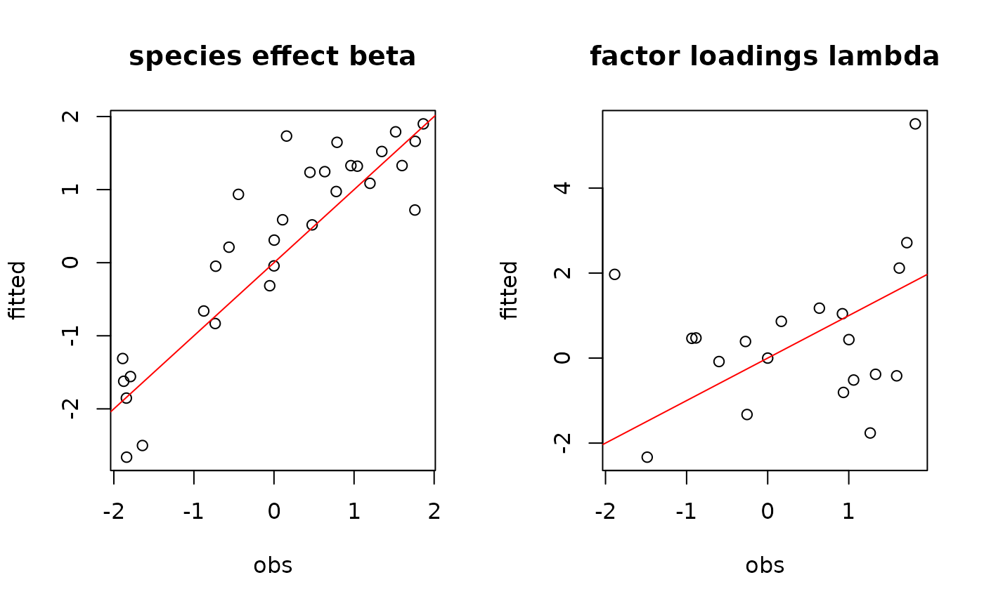
# Species effects beta and factor loadings lambda
par(mfrow=c(1,2))
plot(beta.target, mean_beta,
     main="species effect beta",
     xlab ="obs", ylab ="fitted")
abline(a=0,b=1,col='red')
plot(lambda.target, mean_lambda,
     main="factor loadings lambda",
     xlab ="obs", ylab ="fitted")
abline(a=0,b=1,col='red')


## W latent variables
par(mfrow=c(1,2))
for (l in 1:n_latent) {
  plot(W[,l],
       summary(mod$mcmc.latent[[paste0("lv_",l)]])[[1]][,"Mean"],
       main = paste0("Latent variable W_", l),
       xlab ="obs", ylab ="fitted")
  abline(a=0,b=1,col='red')
}


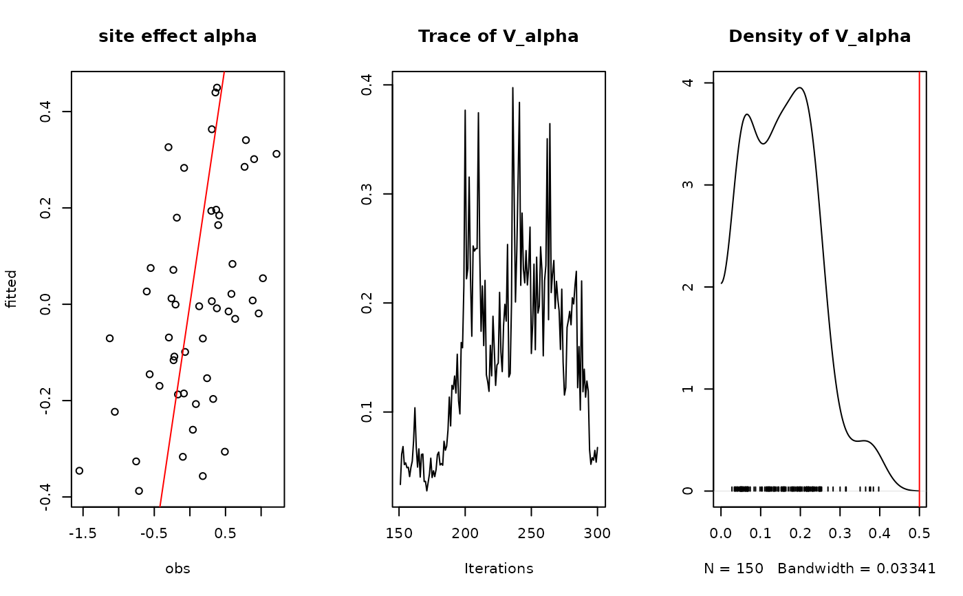
## alpha
par(mfrow=c(1,3))
plot(alpha.target, summary(mod$mcmc.alpha)[[1]][,"Mean"],
     xlab ="obs", ylab ="fitted", main="site effect alpha")
abline(a=0,b=1,col='red')
## Valpha
coda::traceplot(mod$mcmc.V_alpha)
coda::densplot(mod$mcmc.V_alpha)
abline(v=V_alpha.target,col='red')


## Deviance
summary(mod$mcmc.Deviance)
#> 
#> Iterations = 151:300
#> Thinning interval = 1 
#> Number of chains = 1 
#> Sample size per chain = 150 
#> 
#> 1. Empirical mean and standard deviation for each variable,
#>    plus standard error of the mean:
#> 
#>           Mean             SD       Naive SE Time-series SE 
#>        699.266         21.720          1.773          5.062 
#> 
#> 2. Quantiles for each variable:
#> 
#>  2.5%   25%   50%   75% 97.5% 
#> 659.4 686.5 697.7 712.2 743.8 
#> 
plot(mod$mcmc.Deviance)


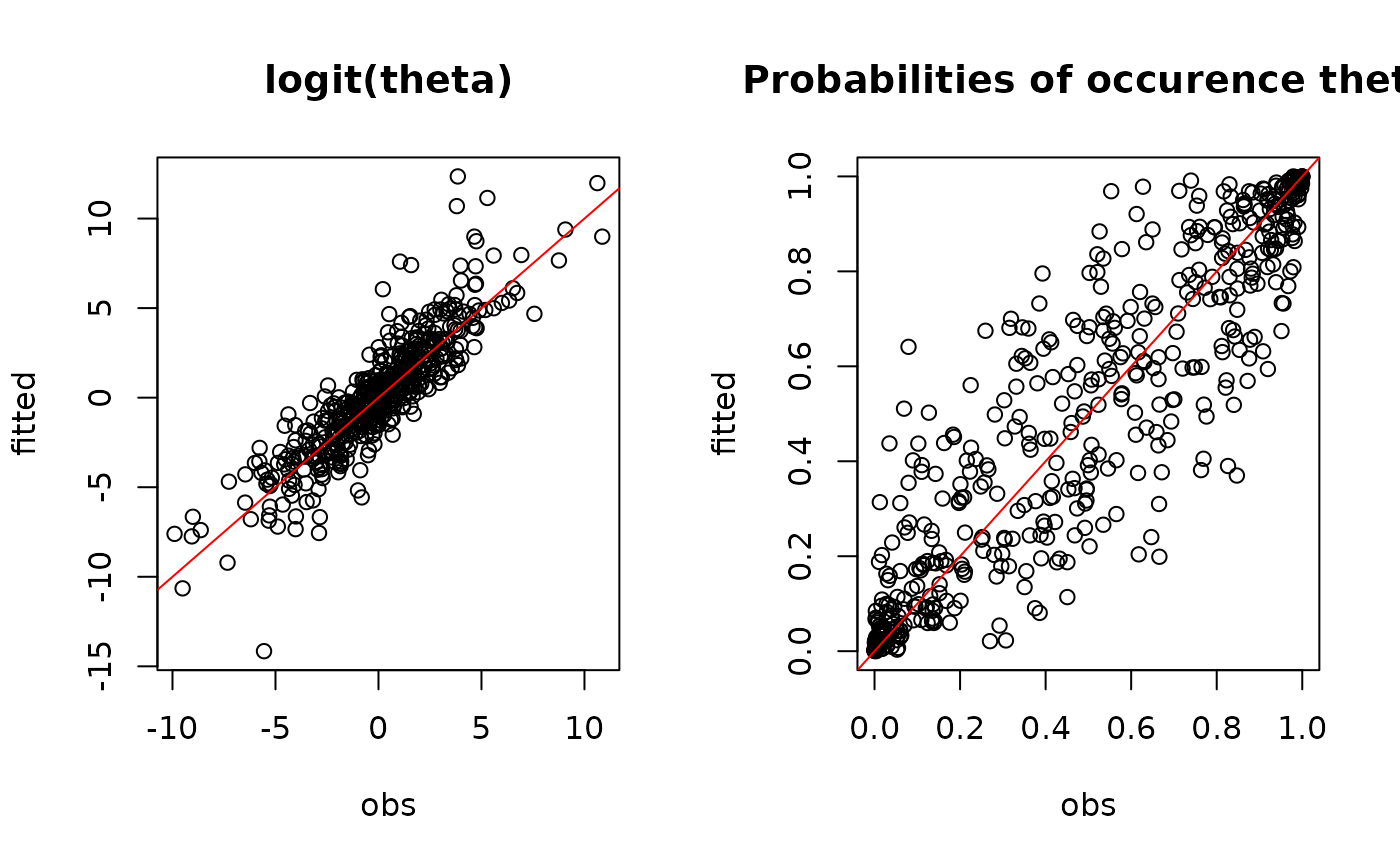
#= Predictions
par(mfrow=c(1,2))
plot(logit.theta, mod$logit_theta_latent,
     main="logit(theta)",
     xlab="obs", ylab="fitted")
abline(a=0 ,b=1, col="red")
plot(theta, mod$theta_latent,
     main="Probabilities of occurence theta",
     xlab="obs", ylab="fitted")
abline(a=0 ,b=1, col="red")

par(oldpar)

if `n_latent=0` and `site_effect="none"`	logit\((\theta_{ij}) = X_i \beta_j\)
if `n_latent>0` and `site_effect="none"`	logit\((\theta_{ij}) = X_i \beta_j + W_i \lambda_j\)
if `n_latent=0` and `site_effect="fixed"`	logit\((\theta_{ij}) = X_i \beta_j + \alpha_i\)
if `n_latent>0` and `site_effect="fixed"`	logit\((\theta_{ij}) = X_i \beta_j + W_i \lambda_j + \alpha_i\)
if `n_latent=0` and `site_effect="random"`	logit\((\theta_{ij}) = X_i \beta_j + \alpha_i\) and \(\alpha_i \sim \mathcal{N}(0,V_\alpha)\)
if `n_latent>0` and `site_effect="random"`	logit\((\theta_{ij}) = X_i \beta_j + W_i \lambda_j + \alpha_i\) and \(\alpha_i \sim \mathcal{N}(0,V_\alpha)\)

	\(x_0\)	\(x_1\)	...	\(x_p\)	...	\(x_{np}\)
	__________	________	________	________	________	________
\(t_0\) \|	\(\gamma_{0,0}\)	\(\gamma_{0,1}\)	...	\(\gamma_{0,p}\)	...	\(\gamma_{0,np}\)	{ effect of
\|	intercept						environmental
\|							variables
\(t_1\) \|	\(\gamma_{1,0}\)	\(\gamma_{1,1}\)	...	\(\gamma_{1,p}\)	...	\(\gamma_{1,np}\)
... \|	...	...	...	...	...	...
\(t_k\) \|	\(\gamma_{k,0}\)	\(\gamma_{k,1}\)	...	\(\gamma_{k,p}\)	...	\(\gamma_{k,np}\)
... \|	...	...	...	...	...	...
\(t_{nt}\) \|	\(\gamma_{nt,0}\)	\(\gamma_{nt,1}\)	...	\(\gamma_{nt,p}\)	...	\(\gamma_{nt,np}\)
	average
	trait effect		interaction	traits	environment