New Caledonia with loss and gain

Get forest cover change from TMF

The function .get_fcc_loss_gain() can be used to download forest cover change from the Tropical Moist Forest product.

This function considers both forest loss and gain (or regrowth) to derive the forest cover change map.

We will use New Caledonia as a case study.

from pathlib import Path
import time

import ee
import geefcc
import numpy as np
import pandas as pd
from tabulate import tabulate

# Initialize GEE
ee.Initialize(project="deforisk", opt_url="https://earthengine-highvolume.googleapis.com")

We want to estimate and map the forest cover change for the period 2015–2025, considering regrowth of at least 5 years as being forest, which is debatable [Bourgoin et al., 2024, Poorter et al., 2016].

# Download data from GEE
min_years = 5
out_dir = Path(f"out_tmf_{min_years}yr")
ofile = out_dir / "fcc_tmf.tif"
if not ofile.is_file():
    start_time = time.time()
    geefcc.get_fcc_loss_gain(
        aoi=(163.5, -23, 168.15, -19.51),
        year1=2015,
        year2=2025,
        min_years=min_years,
        tile_size=1,
        crop_to_aoi=True,
        parallel=True,
        output_file=ofile,
    )
    end_time = time.time()

We estimate the computation time to download 20 1-degree tiles using several cores.

elapsed_time = (end_time - start_time) / 60
print('Execution time:', round(elapsed_time, 2), 'minutes')

Execution time: 1.19 minutes

Plot the forest cover change map

We plot the forest cover change map. The raster is automatically resampled to a coarser resolution before plotting as it exceeds the default pixel threshold. Country borders and the tile grid are overlaid directly from their vector files.

geefcc.plot_fcc_loss_gain(
    input_file=ofile,
    output_file=f"fcc_tmf_{min_years}yr.png",
    title="Forest cover change 2015-2025, TMF",
    dpi=200,
    borders=Path("data") / "borders_NCL.gpkg",
    grid=out_dir / "grid.gpkg",
    xlim=(163, 169),
    ylim=(-23.25, -18.75),
)

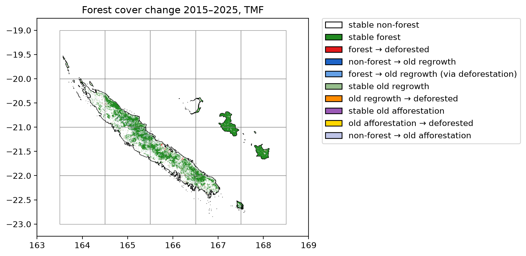
Lines in black represent country borders. One degree tiles in grey cover the whole buffer and were used to download the data in parallel.

Area per class of forest cover change

We use function stat_fcc_loss_gain() to reproject the raster and compute the number of pixels per class and the corresponding area (in ha). We use projection UTM zone 58S (EPSG code 32758) for New Caledonia.

res_df = geefcc.stat_fcc_loss_gain(
    input_file=ofile,
    epsg=32758,
    output_file=f"fcc_statistics_{min_years}yr.csv",
)
tabulate(res_df, headers=res_df.columns, tablefmt="orgtbl", showindex=False)

category	label	count	area_ha
0	stable non-forest	200532616	18047935
1	stable forest	9349449	841450
2	forest –> deforested	161223	14510
3	non-forest –> old regrowth	781232	70311
4	forest –> old regrowth (via deforestation)	16623	1496
5	stable old-regrowth	516513	46486
6	old regrowth –> deforested	9192	827

Deforestation and regrowth estimates

We can then estimate gross loss, gross gain and net loss in forest cover change for the period 2015–2025. Category 4 (forest –> old regrowth via deforestation) is accounted for both gross loss and gain.

forest_t1 = res_df.loc[[1, 2, 4, 5, 6], "area_ha"].sum()
forest_t2 = res_df.loc[[1, 3, 4, 5], "area_ha"].sum()
gross_loss = - res_df.loc[[2, 4, 6], "area_ha"].sum()
gross_gain = res_df.loc[[3, 4], "area_ha"].sum()
lossgain_df = pd.DataFrame({
    "label": ["forest_t1", "forest_t2", "gross loss", "gross gain", "net change"],
    "area_ha": [forest_t1, forest_t2, gross_loss, gross_gain, gross_gain + gross_loss],
})
time = 2025 - 2015
lossgain_df["annual_change_ha"] = (lossgain_df["area_ha"] / time).round().astype(int)
ratio = lossgain_df["area_ha"] / forest_t1
lossgain_df["annual_change_perc"] = round(100 * (1 - pow((1 - ratio), 1 / time)), 2)
lossgain_df.iloc[:2, 2:4] = np.nan

# Export
lossgain_df.to_csv(f"loss_gain_statistics_{min_years}yr.csv", index=False)
tabulate(lossgain_df, headers=lossgain_df.columns, tablefmt="orgtbl", showindex=False)

label	area_ha	annual_change_ha	annual_change_perc
forest_t1	904769	nan	nan
forest_t2	959743	nan	nan
gross loss	-16833	-1683	-0.18
gross gain	71807	7181	0.82
net change	54974	5497	0.62

When considering regrowth of at least 5 years, which is very short for forest recovery [Bourgoin et al., 2024], the gain (7181 ha/yr) compensates the forest cover loss (-1683 ha/yr), and the net change is positive (5947 ha/yr).

If we consider regrowth of at least 10 years as being forest (min_years=10 in function get_fcc_loss_gain), the gain is much smaller (4342 ha/yr), but the net change is still positive (2728 ha/yr corresponding to 0.32 %/yr).

References

[1] (1,2)

C. Bourgoin, G. Ceccherini, M. Girardello, C. Vancutsem, V. Avitabile, P. S. A. Beck, R. Beuchle, L. Blanc, G. Duveiller, M. Migliavacca, G. Vieilledent, A. Cescatti, and F. Achard. Human degradation of tropical moist forests is greater than previously estimated. Nature, 631(8021):570–576, July 2024. doi:10.1038/s41586-024-07629-0.

[2]

L. Poorter, F. Bongers, T. M. Aide, A. M. Almeyda Zambrano, P. Balvanera, J. M. Becknell, V. Boukili, P. H. S. Brancalion, E. N. Broadbent, R. L. Chazdon, D. Craven, J. S. de Almeida-Cortez, G. A. L. Cabral, B. H. J. de Jong, J. S. Denslow, D. H. Dent, S. J. DeWalt, J. M. Dupuy, S. M. Durán, M. M. Espírito-Santo, M. C. Fandino, R. G. César, J. S. Hall, J. L. Hernandez-Stefanoni, C. C. Jakovac, A. B. Junqueira, D. Kennard, S. G. Letcher, J.-C. Licona, M. Lohbeck, E. Marín-Spiotta, M. Martínez-Ramos, P. Massoca, J. A. Meave, R. Mesquita, F. Mora, R. Muñoz, R. Muscarella, Y. R. F. Nunes, S. Ochoa-Gaona, A. A. de Oliveira, E. Orihuela-Belmonte, M. Peña-Claros, E. A. Pérez-García, D. Piotto, J. S. Powers, J. Rodríguez-Velázquez, I. E. Romero-Pérez, J. Ruíz, J. G. Saldarriaga, A. Sanchez-Azofeifa, N. B. Schwartz, M. K. Steininger, N. G. Swenson, M. Toledo, M. Uriarte, M. van Breugel, H. van der Wal, M. D. M. Veloso, H. F. M. Vester, A. Vicentini, I. C. G. Vieira, T. V. Bentos, G. B. Williamson, and D. M. A. Rozendaal. Biomass resilience of neotropical secondary forests. Nature, 530(7589):211–214, February 2016. doi:10.1038/nature16512.