Loss and gain¶

Get forest cover change from TMF¶

The function .get_fcc_loss_gain() can be used to download the forest cover change from the Tropical Moist Forest product.

This function, contrary to get_fcc_loss() which accounts only for loss in the forest cover change, considers both forest loss and gain (also called regrowth) to derive the forest cover change map.

We will use the Reunion Island (isocode “REU”) as a case study.

import os

import ee
import geefcc
import numpy as np
import pandas as pd
from tabulate import tabulate

# Some convenient aliases
opj = os.path.join

# Initialize GEE
ee.Initialize(project="deforisk", opt_url="https://earthengine-highvolume.googleapis.com")

We want to estimate and map the forest cover change for the period 2015–2025, considering regrowth of at least 5 years as being forest, which is debatable [Bourgoin et al., 2024, Poorter et al., 2016].

# Download data from GEE
out_dir = "out_tmf_5yr"
ofile = opj(out_dir, "fcc_tmf.tif")
if not os.path.isfile(ofile):
    geefcc.get_fcc_loss_gain(
        aoi="REU",
        year1=2015,
        year2=2025,
        min_years=5,
        tile_size=0.5,
        crop_to_aoi=True,
        parallel=True,
        output_file=ofile,
    )

Plot the forest cover change map¶

geefcc.plot_fcc_loss_gain(
    input_file=ofile,
    output_file="fcc_loss_gain.png",
    title="Forest cover change 2015-2025, TMF",
    dpi=100,
)

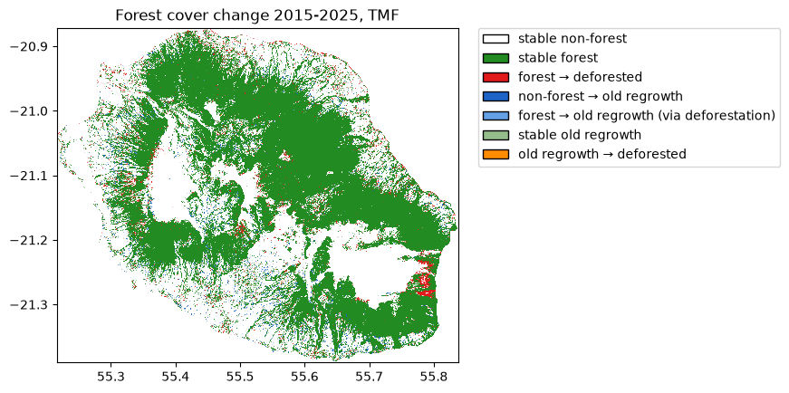
Area per class of forest cover change¶

We use function fcc_area() to reproject the raster and compute the number of pixels per class and the corresponding area (in ha). We use projection UTM zone 40S (EPSG code 32740) for Reunion island.

res_df = geefcc.stat_fcc_loss_gain(
    input_file=ofile,
    epsg=32740,
    output_file="fcc_statistics.csv",
)
tabulate(res_df, headers=res_df.columns, tablefmt="orgtbl", showindex=False)

**Area per class of forest cover change.** A regrowth is considered “old” in this example if it has at least 5 years.¶
category	label	count	area_ha
0	stable non-forest	2672678	240541
1	stable forest	1387668	124890
2	forest –> deforested	67986	6119
3	non-forest –> old regrowth	49882	4489
4	forest –> old regrowth (via deforestation)	1057	95
5	stable old-regrowth	14629	1317
6	old regrowth –> deforested	946	85

Deforestation and regrowth estimates¶

We can then estimate gross loss, gross gain and net loss in forest cover change for the period 2015–2025. Category 4 (forest –> old regrowth via deforestation) is accounted for both gross loss and gain.

forest_t1 = res_df.loc[[1, 2, 4, 5, 6], "area_ha"].sum()
forest_t2 = res_df.loc[[1, 3, 4, 5], "area_ha"].sum()
gross_loss = - res_df.loc[[2, 4, 6], "area_ha"].sum()
gross_gain = res_df.loc[[3, 4], "area_ha"].sum()
lossgain_df = pd.DataFrame({
    "label": ["forest_t1", "forest_t2", "gross loss", "gross gain", "net change"],
    "area_ha": [forest_t1, forest_t2, gross_loss, gross_gain, gross_gain + gross_loss],
})
time = 2025 - 2015
lossgain_df["annual_change_ha"] = (lossgain_df["area_ha"] / time).round().astype(int)
ratio = lossgain_df["area_ha"] / forest_t1
lossgain_df["annual_change_perc"] = round(100 * (1 - pow((1 - ratio), 1 / time)), 2)
lossgain_df.iloc[:2, 2:4] = np.nan

# Export
lossgain_df.to_csv(opj("loss_gain_statistics.csv"), index=False)
tabulate(lossgain_df, headers=lossgain_df.columns, tablefmt="orgtbl", showindex=False)

label	area_ha	annual_change_ha	annual_change_perc
forest_t1	132506	nan	nan
forest_t2	130791	nan	nan
gross loss	-6299	-630	-0.47
gross gain	4584	458	0.35
net change	-1715	-172	-0.13

When considering regrowth of at least 5 years, which is very short for forest recovery [Bourgoin et al., 2024], the gain (458 ha/yr) compensates the forest cover loss (-630 ha/yr), and the net deforestation is small (-172 ha/yr).

If we consider regrowth of at least 10 years as being forest (min_years=10 in function get_fcc_loss_gain), the gain is much smaller (202 ha/yr) and the net deforestation much higher (-427 ha/yr corresponding to -0.32 %/yr).

References¶

[1] (1,2)

C. Bourgoin, G. Ceccherini, M. Girardello, C. Vancutsem, V. Avitabile, P. S. A. Beck, R. Beuchle, L. Blanc, G. Duveiller, M. Migliavacca, G. Vieilledent, A. Cescatti, and F. Achard. Human degradation of tropical moist forests is greater than previously estimated. Nature, 631(8021):570–576, July 2024. doi:10.1038/s41586-024-07629-0.

[2]

L. Poorter, F. Bongers, T. M. Aide, A. M. Almeyda Zambrano, P. Balvanera, J. M. Becknell, V. Boukili, P. H. S. Brancalion, E. N. Broadbent, R. L. Chazdon, D. Craven, J. S. de Almeida-Cortez, G. A. L. Cabral, B. H. J. de Jong, J. S. Denslow, D. H. Dent, S. J. DeWalt, J. M. Dupuy, S. M. Durán, M. M. Espírito-Santo, M. C. Fandino, R. G. César, J. S. Hall, J. L. Hernandez-Stefanoni, C. C. Jakovac, A. B. Junqueira, D. Kennard, S. G. Letcher, J.-C. Licona, M. Lohbeck, E. Marín-Spiotta, M. Martínez-Ramos, P. Massoca, J. A. Meave, R. Mesquita, F. Mora, R. Muñoz, R. Muscarella, Y. R. F. Nunes, S. Ochoa-Gaona, A. A. de Oliveira, E. Orihuela-Belmonte, M. Peña-Claros, E. A. Pérez-García, D. Piotto, J. S. Powers, J. Rodríguez-Velázquez, I. E. Romero-Pérez, J. Ruíz, J. G. Saldarriaga, A. Sanchez-Azofeifa, N. B. Schwartz, M. K. Steininger, N. G. Swenson, M. Toledo, M. Uriarte, M. van Breugel, H. van der Wal, M. D. M. Veloso, H. F. M. Vester, A. Vicentini, I. C. G. Vieira, T. V. Bentos, G. B. Williamson, and D. M. A. Rozendaal. Biomass resilience of neotropical secondary forests. Nature, 530(7589):211–214, February 2016. doi:10.1038/nature16512.

geefcc

Navigation

Related Topics