Large countries

Download the data from GEE

We can use geefcc to download forest cover change for large countries, for example Perou (iso code “PER”). The country will be divided into several tiles which are processed in parallel. If your computer has n cores, n-1 cores will be used in parallel.

import os
import time

import ee
import numpy as np
from osgeo import gdal
from geefcc import get_fcc, sum_raster_bands
import geopandas
import matplotlib.pyplot as plt
from matplotlib.colors import ListedColormap
import matplotlib.patches as mpatches

We initialize Google Earth Engine.

# Initialize GEE
ee.Initialize(project="forestatrisk",
              opt_url=("https://earthengine-highvolume."
                       "googleapis.com"))

We can compute the number of cores used for the computation.

ncpu = os.cpu_count() - 1
ncpu

3

We download the forest cover change data from GEE for Peru for years 2000, 2010 and 2020, using a buffer of about 10 km around the border (0.089… decimal degrees) and a tile size of one degree.

A buffer can be useful if we want to avoid “edge effects”, while computing distance to forest edge for example. One degree tiles are used to download the data from GEE in parallel.

start_time = time.time()
get_fcc(
    aoi="PER",
    buff=0.08983152841195216,
    years=[2000, 2010, 2020],
    source="tmf",
    tile_size=1,
    output_file="out_tmf/forest_tmf.tif",
)
end_time = time.time()

We estimate the computation time to download 159 1-degree tiles using several cores.

elapsed_time = (end_time - start_time) / 60
print('Execution time:', round(elapsed_time, 2), 'minutes')

Execution time: 30.76 minutes

Transform multiband fcc raster in one band raster

We transform the data to have only one band describing the forest cover change with 0 for non-forest, 1 for deforestation on the period 2000–2009, 2 for deforestation on the period 2010–2019, and 3 for the remaining forest in 2020. To do so, we just sum the values of the raster bands.

sum_raster_bands(input_file="out_tmf/forest_tmf.tif",
                 output_file="out_tmf/fcc_tmf.tif",
                 verbose=False)

We resample at a lower resolution for plotting.

infn = "out_tmf/fcc_tmf.tif"
outfn = "out_tmf/fcc_tmf_coarsen.tif"
scale = gdal.Open(infn).GetGeoTransform()[1]
xres = 20 * scale
yres = 20 * scale
resample_alg = "near"

ds = gdal.Warp(outfn, infn, xRes=xres, yRes=yres, resampleAlg=resample_alg)
ds = None

Plot the forest cover change map

We prepare the colors for the map.

# Colors
cols=[(255, 165, 0, 255), (227, 26, 28, 255), (34, 139, 34, 255)]
colors = [(1, 1, 1, 0)]  # transparent white for 0
cmax = 255.0  # float for division
for col in cols:
    col_class = tuple([i / cmax for i in col])
    colors.append(col_class)
color_map = ListedColormap(colors)

# Labels
labels = {0: "non-forest in 2000", 1:"deforestation 2000-2009",
          2:"deforestation 2010-2019", 3:"forest in 2020"}
patches = [mpatches.Patch(facecolor=col, edgecolor="black",
                          label=labels[i]) for (i, col) in enumerate(colors)]

We load the data: country borders, buffer, and grid.

# Borders
borders_gpkg = os.path.join("out_tmf", "gadm41_PER_0.gpkg")
borders = geopandas.read_file(borders_gpkg)

# Buffer
buffer_gpkg = os.path.join("out_tmf", "gadm41_PER_buffer.gpkg")
buffer = geopandas.read_file(buffer_gpkg)

# Grid
grid_gpkg = os.path.join("out_tmf", "min_grid.gpkg")
grid = geopandas.read_file(grid_gpkg)

We plot the forest cover change map.

with gdal.Open("out_tmf/fcc_tmf_coarsen.tif", gdal.GA_ReadOnly) as ds:
    raster_image = ds.ReadAsArray()
    nrow, ncol = raster_image.shape
    xmin, xres, _, ymax, _, yres = ds.GetGeoTransform()
    extent = [xmin, xmin + xres * ncol, ymax + yres * nrow, ymax]

# Plot
fig = plt.figure()
ax = plt.subplot(111)
ax.imshow(raster_image, cmap=color_map, extent=extent,
          resample=False)
grid_image = grid.boundary.plot(ax=ax, color="grey", linewidth=0.5)
borders_image = borders.boundary.plot(ax=ax, color="black", linewidth=0.5)
buffer_image = buffer.boundary.plot(ax=ax, color="black", linewidth=0.5)
plt.title("Forest cover change 2000-2010-2020, TMF")
plt.legend(handles=patches, bbox_to_anchor=(1.05, 1), loc=2, borderaxespad=0.)
fig.savefig("fcc.png", bbox_inches="tight", dpi=200)

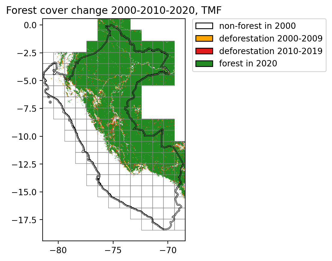
Lines in black represent country borders and the 10 km buffer. One degree tiles in grey cover the whole buffer and were used to download the data in parallel.