New Caledonia¶

Downloading data in parallel¶

We can use geefcc to download forest cover change for large countries, for example New-Caledonia. The country will be divided into several tiles which are processed in parallel. If your computer has n cores, n-1 cores will be used in parallel.

import os
import time

import ee
import numpy as np
import pandas as pd
from osgeo import gdal
from geefcc import get_fcc, sum_raster_bands
import geopandas
import matplotlib.pyplot as plt
from matplotlib.colors import ListedColormap
import matplotlib.patches as mpatches
from tabulate import tabulate

We initialize Google Earth Engine.

# Initialize GEE
ee.Initialize(project="deforisk",
              opt_url=("https://earthengine-highvolume."
                       "googleapis.com"))

We can compute the number of cores used for the computation.

ncpu = os.cpu_count() - 1
ncpu

Using TMF product¶

Downloading data¶

We download the forest cover change data from GEE for New Caledonia for years 2001, 2010 and 2020, using a tile size of one degree. We use the TMF product (version v1_2025 available in geefcc).

start_time = time.time()
get_fcc(
    aoi=(163.5, -23, 168.15, -19.51),
    buff=0.0,
    years=[2001, 2010, 2020],
    source="tmf",
    tile_size=1.0,
    crop_to_aoi=True,
    output_file="out_tmf/forest_tmf.tif",
    parallel=True,
    ncpu=ncpu)
end_time = time.time()

get_fcc running, 20 tiles .....................

We estimate the computation time to download 20 1-degree tiles using several cores.

elapsed_time = (end_time - start_time) / 60
print('Execution time:', round(elapsed_time, 2), 'minutes')

Execution time: 1.2 minutes

Transform multiband fcc raster in one band raster¶

We transform the data to have only one band describing the forest cover change with 0 for non-forest, 1 for deforestation on the period 2000–2009, 2 for deforestation on the period 2010–2019, and 3 for the remaining forest in 2020. To do so, we just sum the values of the raster bands.

sum_raster_bands(input_file="out_tmf/forest_tmf.tif",
                 output_file="out_tmf/fcc_tmf.tif",
                 verbose=False)

We resample at a lower resolution for plotting.

infn = "out_tmf/fcc_tmf.tif"
outfn = "out_tmf/fcc_tmf_coarsen.tif"
scale = gdal.Open(infn).GetGeoTransform()[1]
xres = 20 * scale
yres = 20 * scale
resample_alg = "near"

ds = gdal.Warp(outfn, infn, xRes=xres, yRes=yres, resampleAlg=resample_alg)
ds = None

Plot the forest cover change map¶

We prepare the colors for the map.

# Colors
cols=[(255, 165, 0, 255), (227, 26, 28, 255), (34, 139, 34, 255)]
colors = [(1, 1, 1, 0)]  # transparent white for 0
cmax = 255.0  # float for division
for col in cols:
    col_class = tuple([i / cmax for i in col])
    colors.append(col_class)
color_map = ListedColormap(colors)

# Labels
labels = {0: "non-forest in 2001", 1:"deforestation 2001-2009",
          2:"deforestation 2010-2019", 3:"forest in 2020"}
patches = [mpatches.Patch(facecolor=col, edgecolor="black",
                          label=labels[i]) for (i, col) in enumerate(colors)]

We created a short function to plot the forest cover change map.

def plot_fcc(title, out_file):
    fig = plt.figure()
    ax = plt.subplot(111)
    ax.imshow(raster_image, cmap=color_map, extent=extent,
              resample=False)
    ax.set_aspect("equal")
    grid_image = grid.boundary.plot(ax=ax, color="grey", linewidth=0.5)
    borders_image = borders.boundary.plot(ax=ax, color="black", linewidth=0.5)
    plt.title(title)
    plt.legend(handles=patches, bbox_to_anchor=(1.05, 1), loc=2, borderaxespad=0.)
    plt.xlim((163, 169))
    plt.ylim((-23.25, -18.75))
    fig.savefig(out_file, bbox_inches="tight", dpi=200)
    plt.close(fig)

We load the data: country borders and grid. The borders can be downloaded from the gadm website.

# Borders
borders_gpkg = os.path.join("data", "borders_NCL.gpkg")
borders = geopandas.read_file(borders_gpkg)

# Grid
grid_gpkg = os.path.join("out_tmf", "grid.gpkg")
grid = geopandas.read_file(grid_gpkg)

We plot the forest cover change map.

with gdal.Open("out_tmf/fcc_tmf_coarsen.tif", gdal.GA_ReadOnly) as ds:
    raster_image = ds.ReadAsArray()
    nrow, ncol = raster_image.shape
    xmin, xres, _, ymax, _, yres = ds.GetGeoTransform()
    extent = [xmin, xmin + xres * ncol, ymax + yres * nrow, ymax]
    plot_fcc("Forest cover change 2001-2010-2020, TMF", "fcc_tmf.png")

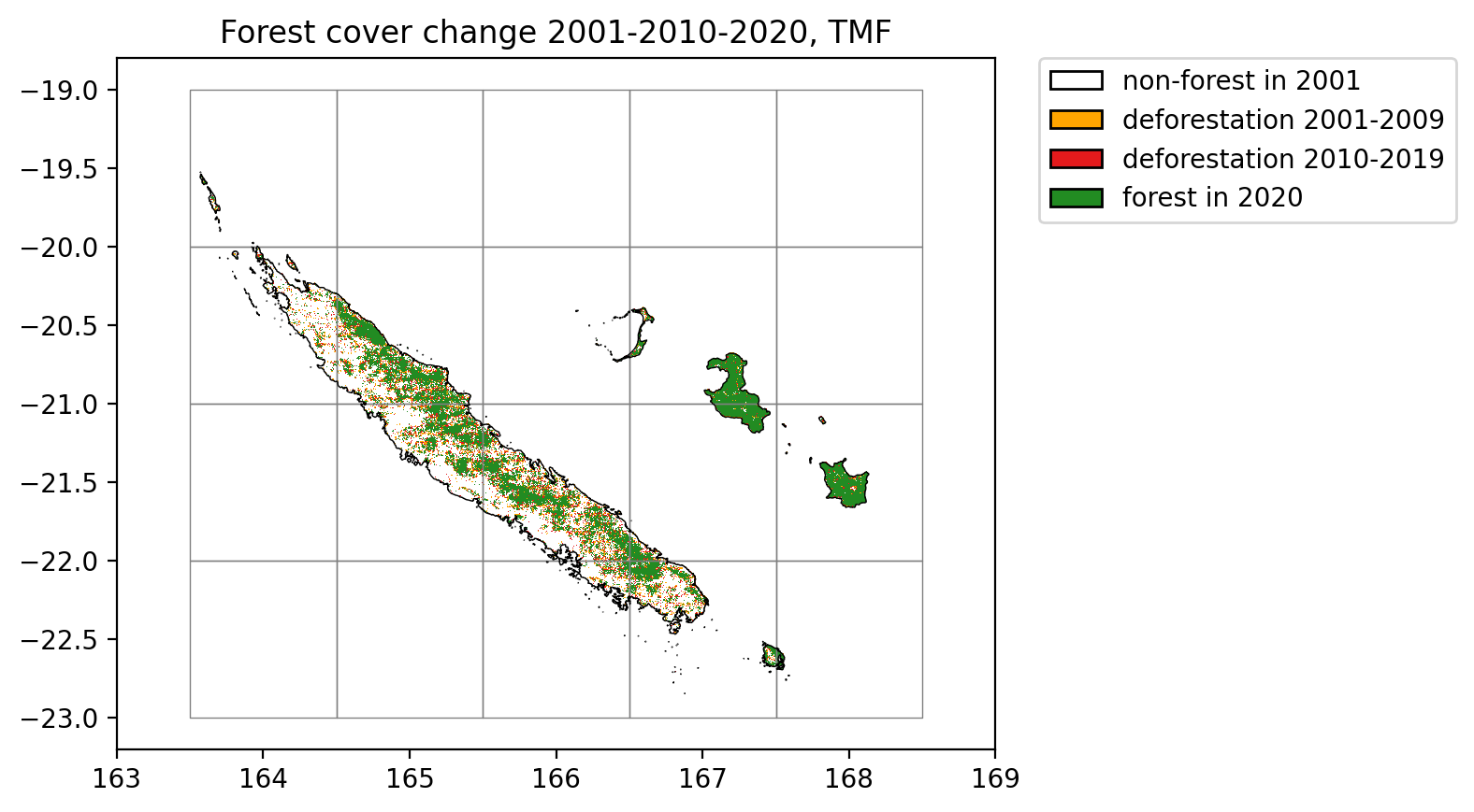
Lines in black represent country borders. One degree tiles in grey cover the whole buffer and were used to download the data in parallel.

Reproject in EPSG:3163 for area computation¶

ifile = os.path.join("out_tmf", "fcc_tmf.tif")
ofile = os.path.join("out_tmf", "fcc_tmf_epsg3163.tif")
ds = gdal.Warp(ofile, ifile, xRes=30, yRes=30, dstSRS="EPSG:3163", resampleAlg="near",
          targetAlignedPixels=True, creationOptions=["COMPRESS=DEFLATE"])
ds = None

Compute statistics¶

We use the tool “Raster layer unique values report” in QGIS to get the number of pixels per pixel value in the raster.

pixel_count = [n1, n2, n3] = [291545, 258015, 9381325]
areas = [round(i * (30 * 30 / 10000)) for i in pixel_count]
tmf_areas= {"product": "tmf", "version": "v1_2025", "perc": "",
 "fc2001": areas[0] + areas[1] + areas[2],
 "fc2010": areas[1] + areas[2], "fc2020": areas[2],
 "d1": round(areas[0] / 9), "d2": round(areas[1] / 10)}
print(tmf_areas)

{'product': 'tmf', 'version': 'v1_2025', 'perc': '', 'fc2001': 893779, 'fc2010': 867540, 'fc2020': 844319, 'd1': 2915, 'd2': 2322}

Using GFC product and tree cover \(\ge\) 80%¶

Downloading data¶

We download the forest cover change data from GEE for New Caledonia for years 2001, 2010 and 2020, using a tile size of one degree. We use the GFC product (version v1_11 available in geefcc) and a tree cover percentage \(\ge\) 80 to define the forest.

start_time = time.time()
get_fcc(
    aoi=(163.5, -23, 168.15, -19.51),
    buff=0.0,
    years=[2001, 2010, 2020],
    source="gfc",
    perc=80,
    tile_size=1.0,
    crop_to_aoi=True,
    output_file="out_gfc80/forest_gfc80.tif",
    parallel=True,
    ncpu=ncpu)
end_time = time.time()

We estimate the computation time to download 20 1-degree tiles using several cores.

elapsed_time = (end_time - start_time) / 60
print('Execution time:', round(elapsed_time, 2), 'minutes')

Execution time: 1.0 minutes

Transform multiband fcc raster in one band raster¶

We transform the data to have only one band describing the forest cover change with 0 for non-forest, 1 for deforestation on the period 2001–2009, 2 for deforestation on the period 2010–2019, and 3 for the remaining forest in 2020. To do so, we just sum the values of the raster bands.

sum_raster_bands(input_file="out_gfc80/forest_gfc80.tif",
                 output_file="out_gfc80/fcc_gfc80.tif",
                 verbose=False)

We resample at a lower resolution for plotting.

infn = "out_gfc80/fcc_gfc80.tif"
outfn = "out_gfc80/fcc_gfc80_coarsen.tif"
scale = gdal.Open(infn).GetGeoTransform()[1]
xres = 20 * scale
yres = 20 * scale
resample_alg = "near"

ds = gdal.Warp(outfn, infn, xRes=xres, yRes=yres, resampleAlg=resample_alg)
ds = None

Plot the forest cover change map¶

We prepare the colors for the map.

# Colors
cols=[(255, 165, 0, 255), (227, 26, 28, 255), (34, 139, 34, 255)]
colors = [(1, 1, 1, 0)]  # transparent white for 0
cmax = 255.0  # float for division
for col in cols:
    col_class = tuple([i / cmax for i in col])
    colors.append(col_class)
color_map = ListedColormap(colors)

# Labels
labels = {0: "non-forest in 2001", 1:"deforestation 2001-2009",
          2:"deforestation 2010-2019", 3:"forest in 2020"}
patches = [mpatches.Patch(facecolor=col, edgecolor="black",
                          label=labels[i]) for (i, col) in enumerate(colors)]

We plot the forest cover change map.

with gdal.Open("out_gfc80/fcc_gfc80_coarsen.tif", gdal.GA_ReadOnly) as ds:
    raster_image = ds.ReadAsArray()
    nrow, ncol = raster_image.shape
    xmin, xres, _, ymax, _, yres = ds.GetGeoTransform()
    extent = [xmin, xmin + xres * ncol, ymax + yres * nrow, ymax]
    plot_fcc("Forest cover change 2001-2010-2020, GFC 80%", "fcc_gfc80.png")

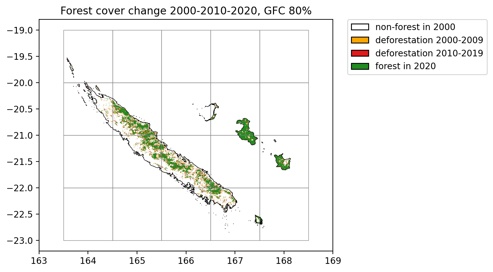
Lines in black represent country borders. One degree tiles in grey cover the whole buffer and were used to download the data in parallel.

Reproject in EPSG:3163 for area computation¶

ifile = os.path.join("out_gfc80", "fcc_gfc80.tif")
ofile = os.path.join("out_gfc80", "fcc_gfc80_epsg3163.tif")
ds = gdal.Warp(ofile, ifile, xRes=30, yRes=30, dstSRS="EPSG:3163", resampleAlg="near",
          targetAlignedPixels=True, creationOptions=["COMPRESS=DEFLATE"])
ds = None

Compute statistics¶

pixel_count = [n1, n2, n3] = [41624, 27874, 7275205]
areas = [round(i * (30 * 30 / 10000)) for i in pixel_count]
gfc80_areas= {"product": "gfc", "version": "v1_13(2025)", "perc": 80,
 "fc2001": areas[0] + areas[1] + areas[2],
 "fc2010": areas[1] + areas[2], "fc2020": areas[2],
 "d1": round(areas[0] / 9), "d2": round(areas[1] / 10)}
print(gfc80_areas)

{'product': 'gfc', 'version': 'v1_13(2025)', 'perc': 80, 'fc2001': 661023, 'fc2010': 657277, 'fc2020': 654768, 'd1': 416, 'd2': 251}

Using GFC product and tree cover \(\ge\) 60%¶

Downloading data¶

We download the forest cover change data from GEE for New Caledonia for years 2000, 2010 and 2020, using a tile size of one degree. We use the GFC product (version v1_11 available in geefcc) and a tree cover percentage \(\ge\) 60 to define the forest.

start_time = time.time()
get_fcc(
    aoi=(163.5, -23, 168.15, -19.51),
    buff=0.0,
    years=[2001, 2010, 2020],
    source="gfc",
    perc=60,
    tile_size=1.0,
    crop_to_aoi=True,
    output_file="out_gfc60/forest_gfc60.tif",
    parallel=True,
    ncpu=ncpu)
end_time = time.time()

We estimate the computation time to download 20 1-degree tiles using several cores.

elapsed_time = (end_time - start_time) / 60
print('Execution time:', round(elapsed_time, 2), 'minutes')

Execution time: 1.12 minutes

Transform multiband fcc raster in one band raster¶

We transform the data to have only one band describing the forest cover change with 0 for non-forest, 1 for deforestation on the period 2001–2009, 2 for deforestation on the period 2010–2019, and 3 for the remaining forest in 2020. To do so, we just sum the values of the raster bands.

sum_raster_bands(input_file="out_gfc60/forest_gfc60.tif",
                 output_file="out_gfc60/fcc_gfc60.tif",
                 verbose=False)

We resample at a lower resolution for plotting.

infn = "out_gfc60/fcc_gfc60.tif"
outfn = "out_gfc60/fcc_gfc60_coarsen.tif"
scale = gdal.Open(infn).GetGeoTransform()[1]
xres = 20 * scale
yres = 20 * scale
resample_alg = "near"

ds = gdal.Warp(outfn, infn, xRes=xres, yRes=yres, resampleAlg=resample_alg)
ds = None

Plot the forest cover change map¶

We plot the forest cover change map.

with gdal.Open("out_gfc60/fcc_gfc60_coarsen.tif", gdal.GA_ReadOnly) as ds:
    raster_image = ds.ReadAsArray()
    nrow, ncol = raster_image.shape
    xmin, xres, _, ymax, _, yres = ds.GetGeoTransform()
    extent = [xmin, xmin + xres * ncol, ymax + yres * nrow, ymax]
    plot_fcc("Forest cover change 2001-2010-2020, GFC 60%", "fcc_gfc60.png")

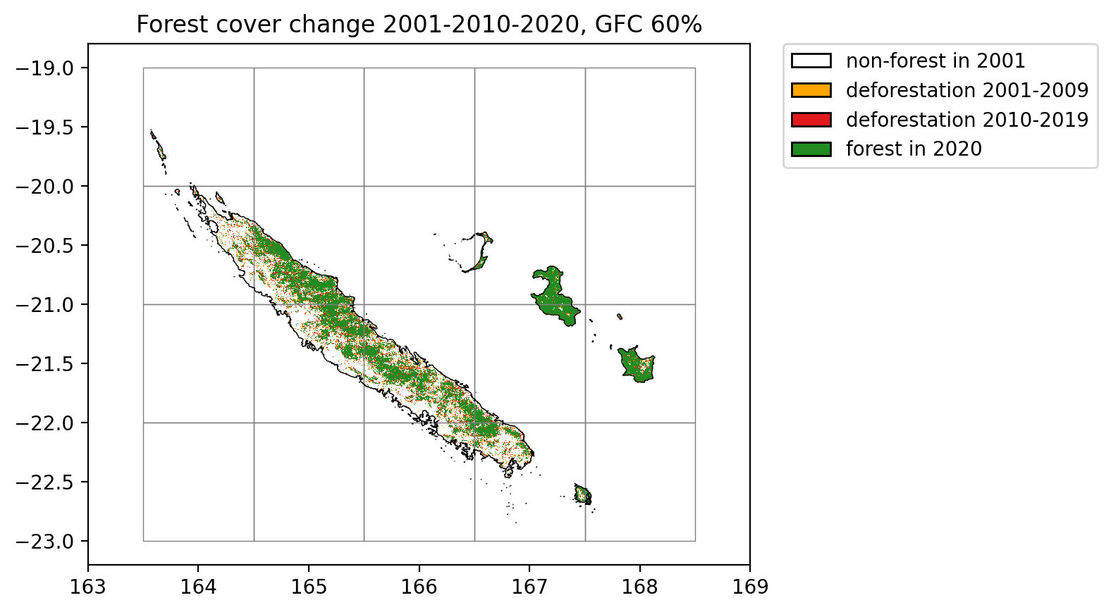
Lines in black represent country borders. One degree tiles in grey cover the whole buffer and were used to download the data in parallel.

Reproject in EPSG:3163 for area computation¶

ifile = os.path.join("out_gfc60", "fcc_gfc60.tif")
ofile = os.path.join("out_gfc60", "fcc_gfc60_epsg3163.tif")
ds = gdal.Warp(ofile, ifile, xRes=30, yRes=30, dstSRS="EPSG:3163", resampleAlg="near",
          targetAlignedPixels=True, creationOptions=["COMPRESS=DEFLATE"])
ds = None

Compute statistics¶

pixel_count = [n1, n2, n3] = [73854, 60386, 9860124]
areas = [round(i * (30 * 30 / 10000)) for i in pixel_count]
gfc60_areas= {"product": "gfc", "version": "v1_13(2025)", "perc": 60,
 "fc2001": areas[0] + areas[1] + areas[2],
 "fc2010": areas[1] + areas[2], "fc2020": areas[2],
 "d1": round(areas[0] / 9), "d2": round(areas[1] / 10)}
print(gfc60_areas)

{'product': 'gfc', 'version': 'v1_13(2025)', 'perc': 60, 'fc2001': 899493, 'fc2010': 892846, 'fc2020': 887411, 'd1': 739, 'd2': 544}

Summary of the results¶

res_df = pd.DataFrame([tmf_areas, gfc80_areas, gfc60_areas])
res_df.to_csv(os.path.join("comparison_geefcc_nc.csv"), index=False)
tabulate(res_df, headers=res_df.columns, tablefmt="orgtbl")

**Comparing forest-cover change products for New Caledonia.** fc: forest cover (in ha), d1: mean annual deforestation (in ha) in the first period 2001–2010, d2: mean annual deforestation (in ha) in the second period 2010–2020, **perc**: tree cover threshold (in %) used to define the forest with GFC.¶
	product	version	perc	fc2001	fc2010	fc2020	d1	d2
0	tmf	v1_2025		893779	867540	844319	2915	2322
1	gfc	v1_13(2025)	80	661023	657277	654768	416	251
2	gfc	v1_13(2025)	60	899493	892846	887411	739	544

Forest cover for TMF and GFC with tree cover \(\ge\) 60% are similar in 2020 (about 850,000 ha) but the annual deforestation is 4-5 times lower when using the GFC product (e.g. 544 ha/yr for GFC in the period 2010–2020 against 2322 ha/yr for TMF for the same period).

geefcc

Navigation

Related Topics

New Caledonia¶

Downloading data in parallel¶

Using TMF product¶

Downloading data¶

Transform multiband fcc raster in one band raster¶

Plot the forest cover change map¶

Reproject in EPSG:3163 for area computation¶

Compute statistics¶

Using GFC product and tree cover \(\ge\) 80%¶

Downloading data¶

Transform multiband fcc raster in one band raster¶

Plot the forest cover change map¶

Reproject in EPSG:3163 for area computation¶

Compute statistics¶

Using GFC product and tree cover \(\ge\) 60%¶

Downloading data¶

Transform multiband fcc raster in one band raster¶

Plot the forest cover change map¶

Reproject in EPSG:3163 for area computation¶

Compute statistics¶

Summary of the results¶