All steps
1 Introduction
1.1 Objective
We present here all the steps of the JNR methodology that need to be followed to derive a map of the deforestation risk in a given jurisdiction.
1.2 Importing Python modules
We import the Python modules needed for running the analysis.
# Imports
import os
import pkg_resources

import numpy as np
import matplotlib.pyplot as plt
import pandas as pd
from tabulate import tabulate

import riskmapjnr as rmj
Increase the cache for GDAL to increase computational speed.
# GDAL
os.environ["GDAL_CACHEMAX"] = "1024"
Set the PROJ_LIB environmental variable.
os.environ["PROJ_LIB"] = "/home/ghislain/.pyenv/versions/miniconda3-latest/envs/conda-rmj/share/proj"
Create a directory to save results.
out_dir = "outputs_steps"
rmj.make_dir(out_dir)
1.3 Forest cover change data
We use the Guadeloupe archipelago as a case study. Recent forest cover change data for Guadeloupe is included in the riskmapjnr package. The raster file (fcc123_GLP.tif) includes the following values: 1 for deforestation on the period 2000–2010, 2 for deforestation on the period 2010–2020, and 3 for the remaining forest in 2020. NoData value is set to 0. The first period (2000–2010) will be used for calibration and the second period (2010–2020) will be used for validation. This is the only data we need to derive a map of deforestation risk following the JNR methodology.
fcc_file = pkg_resources.resource_filename("riskmapjnr", "data/fcc123_GLP.tif")
print(fcc_file)
border_file = pkg_resources.resource_filename("riskmapjnr", "data/ctry_border_GLP.gpkg")
print(border_file)
/home/ghislain/Code/riskmapjnr/riskmapjnr/data/fcc123_GLP.tif
/home/ghislain/Code/riskmapjnr/riskmapjnr/data/ctry_border_GLP.gpkg
We plot the forest cover change map with the plot.fcc123() function.
ofile = os.path.join(out_dir, "fcc123.png")
fig_fcc123 = rmj.plot.fcc123(
    input_fcc_raster=fcc_file,
    maxpixels=1e8,
    output_file=ofile,
    borders=border_file,
    linewidth=0.2,
    figsize=(5, 4), dpi=800)
ofile
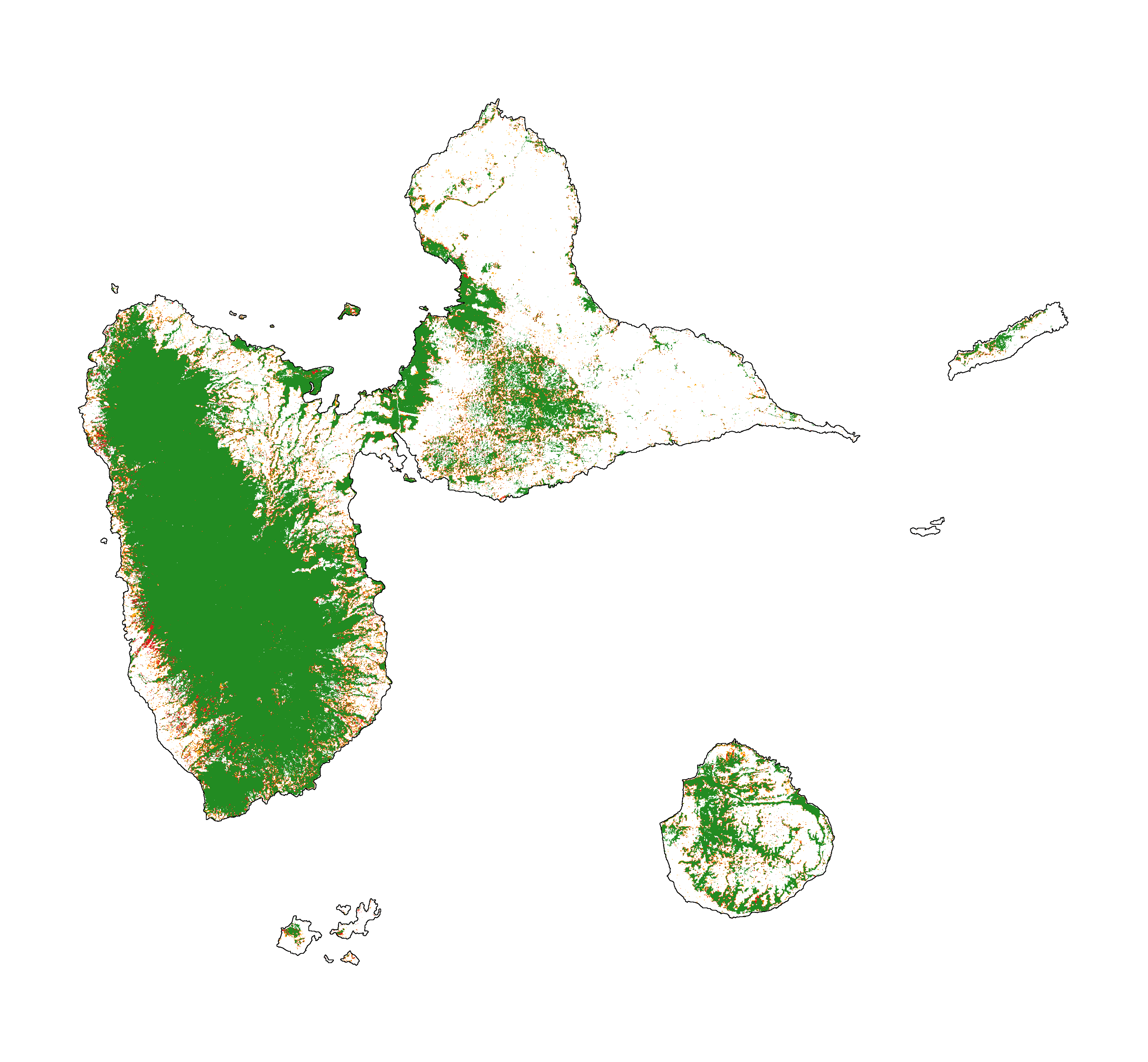
Forest cover change map. Deforestation on the first period (2000–2010) is in orange, deforestation on the second period (2000–2020) is in red and remaining forest (in 2020) is in green.
2 Deforestation risk and distance to forest edge
The first step is to compute the distance to the forest edge after which the risk of deforestation becomes negligible. Indeed, it is known from previous studies on tropical deforestation that the deforestation risk decreases rapidly with the distance to the forest edge and that most of the deforestation occurs close to the forest edge (Vieilledent et al., 2013, Grinand et al., 2020, Vieilledent, 2021, Dezécache et al., 2017). The JNR methodology suggests identifying the distance to the forest edge \(d\), so that at least 99% of the deforestation occurs within a distance \(\leq d\). Forest areas located at a distance from the forest edge \(\gt d\) can be considered as having no risk of being deforested. As a consequence, forest pixels with a distance from the forest edge \(\gt d\) are assigned category 0 (zero) for the deforestation risk.
ofile = os.path.join(out_dir, "perc_dist.png")
dist_edge_thres = rmj.dist_edge_threshold(
    fcc_file=fcc_file,
    defor_values=1,
    dist_file=os.path.join(out_dir, "dist_edge.tif"),
    dist_bins=np.arange(0, 1080, step=30),
    tab_file_dist=os.path.join(out_dir, "tab_dist.csv"),
    fig_file_dist=ofile,
    blk_rows=128, verbose=False)
ofile
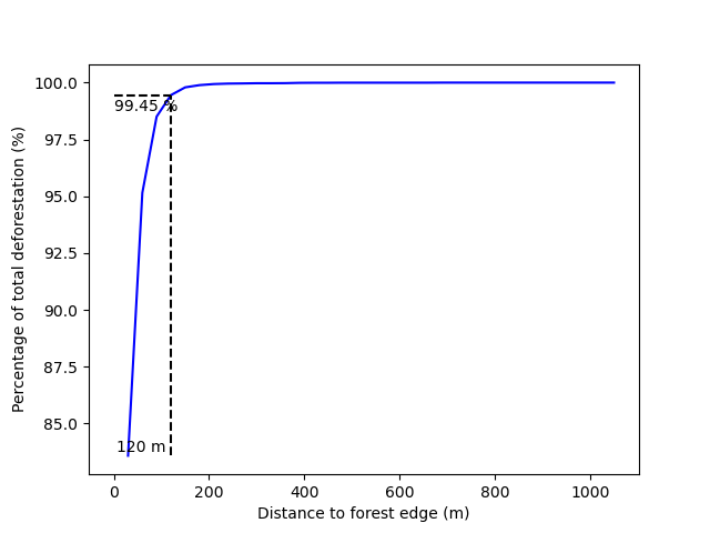
Identifying areas for which the risk of deforestation is negligible. Figure shows that more than 99% of the deforestation occurs within a distance from the forest edge ≤ 120 m. Forest areas located at a distance > 120 m from the forest edge can be considered as having no risk of being deforested.
The function returns a dictionnary including the distance threshold.
dist_thresh = dist_edge_thres["dist_thresh"]
print(f"The distance threshold is {dist_thresh} m")
The distance threshold is 120 m
A table indicating the cumulative percentage of deforestation as a function of the distance is also produced:
Distance |
Npixels |
Area |
Cumulation |
Percentage |
|---|---|---|---|---|
30 |
24937 |
2244.33 |
2244.33 |
83.583 |
60 |
3451 |
310.59 |
2554.92 |
95.15 |
90 |
1001 |
90.09 |
2645.01 |
98.5051 |
120 |
282 |
25.38 |
2670.39 |
99.4503 |
150 |
102 |
9.18 |
2679.57 |
99.7922 |
180 |
29 |
2.61 |
2682.18 |
99.8894 |
210 |
14 |
1.26 |
2683.44 |
99.9363 |
240 |
6 |
0.54 |
2683.98 |
99.9564 |
270 |
2 |
0.18 |
2684.16 |
99.9631 |
300 |
3 |
0.27 |
2684.43 |
99.9732 |
3 Local deforestation rate
The second step is to compute a local risk of deforestation at the pixel level using a moving window made of several pixels. The deforestation risk is estimated from the deforestation rate inside the moving window. The deforestation rate \(\theta\) (in %/yr) is computed from the formula \(\theta=1-(\alpha_2/\alpha_1)^{1/\tau}\), with \(\alpha\) the forest areas (in ha) at time \(t_1\) and \(t_2\), and \(\tau\), the time interval (in yr) between time \(t_1\) and \(t_2\). Using the deforestation rate formula, the moving window and the past forest cover change map, we can derive a raster map describing the local risk of deforestation at the same resolution as the input map.
To save space on disk, deforestation rates are converted to integer values between 1 and 10000 (ten thousand) and the raster type is set to UInt16. This ensures a precision of 10-4for the deforestation rate which is sufficient to determine the 30 categories of deforestation risk, as imposed by the JNR methodology.
# Set window size
s = 5
# Compute local deforestation rate
rmj.local_defor_rate(
    fcc_file=fcc_file,
    defor_values=1,
    ldefrate_file=os.path.join(out_dir, "ldefrate.tif"),
    win_size=s,
    time_interval=10,
    blk_rows=100,
    verbose=False)
4 Pixels with zero risk of deforestation
This third step sets a value of 0 to pixels with zero deforestation risk. Value 65535 will be used for NoData. As explained previously, a risk of deforestation of zero is assumed when distance to forest edge is greater than the distance below which more than 99% of the deforestation occurs.
rmj.set_defor_cat_zero(
    ldefrate_file=os.path.join(out_dir, "ldefrate.tif"),
    dist_file=os.path.join(out_dir, "dist_edge.tif"),
    dist_thresh=dist_thresh,
    ldefrate_with_zero_file=os.path.join(out_dir, "ldefrate_with_zero.tif"),
    blk_rows=128,
    verbose=False)
5 Categories of deforestation risk
The fourth step implies converting the continuous values of the raster map of deforestation risk to categorical values. The JNR methodology suggests to use 31 classes of risk from “0” to “30” including the “0” class for the forest pixels with no risk of being deforested (located at a distance to the forest edge \(> d\), see first step). Following the JNR methodology, at least three slicing algorithms must be compared to derive the categorical map of deforestation risk, such as “equal area”, “equal interval”, and “natural breaks”. With the “equal area” algorithm, each class from “1” to “30” must cover approximately the same area. With the “equal interval” algorithm, classes from “1” to “30” correspond to bins of deforestation risk of the same range. In this case, some risk classes will be in majority in the landscape compared to other classes of lower frequency. With the “natural breaks” algorithm, the continuous deforestation risk is normalized before running an “equal interval” algorithm.
bins = rmj.defor_cat(
    ldefrate_with_zero_file=os.path.join(out_dir, "ldefrate_with_zero.tif"),
    riskmap_file=os.path.join(out_dir, "riskmap.tif"),
    ncat=30,
    method="Equal Interval",
    blk_rows=128,
    verbose=False)
print(f"Bins:\n{bins}")
Bins:
[    0     1   334   668  1001  1334  1668  2001  2334  2667  3001  3334
  3667  4001  4334  4667  5000  5334  5667  6000  6334  6667  7000  7334
  7667  8000  8334  8667  9000  9333  9667 10001]
The risk map can be plotted using the plot.riskmap() function.
ofile = os.path.join(out_dir, "riskmap.png")
riskmap_fig = rmj.plot.riskmap(
    input_risk_map=os.path.join(out_dir, "riskmap.tif"),
    maxpixels=1e8,
    output_file=ofile,
    borders=border_file,
    legend=True,
    figsize=(5, 4), dpi=800,
    linewidth=0.2,)
ofile
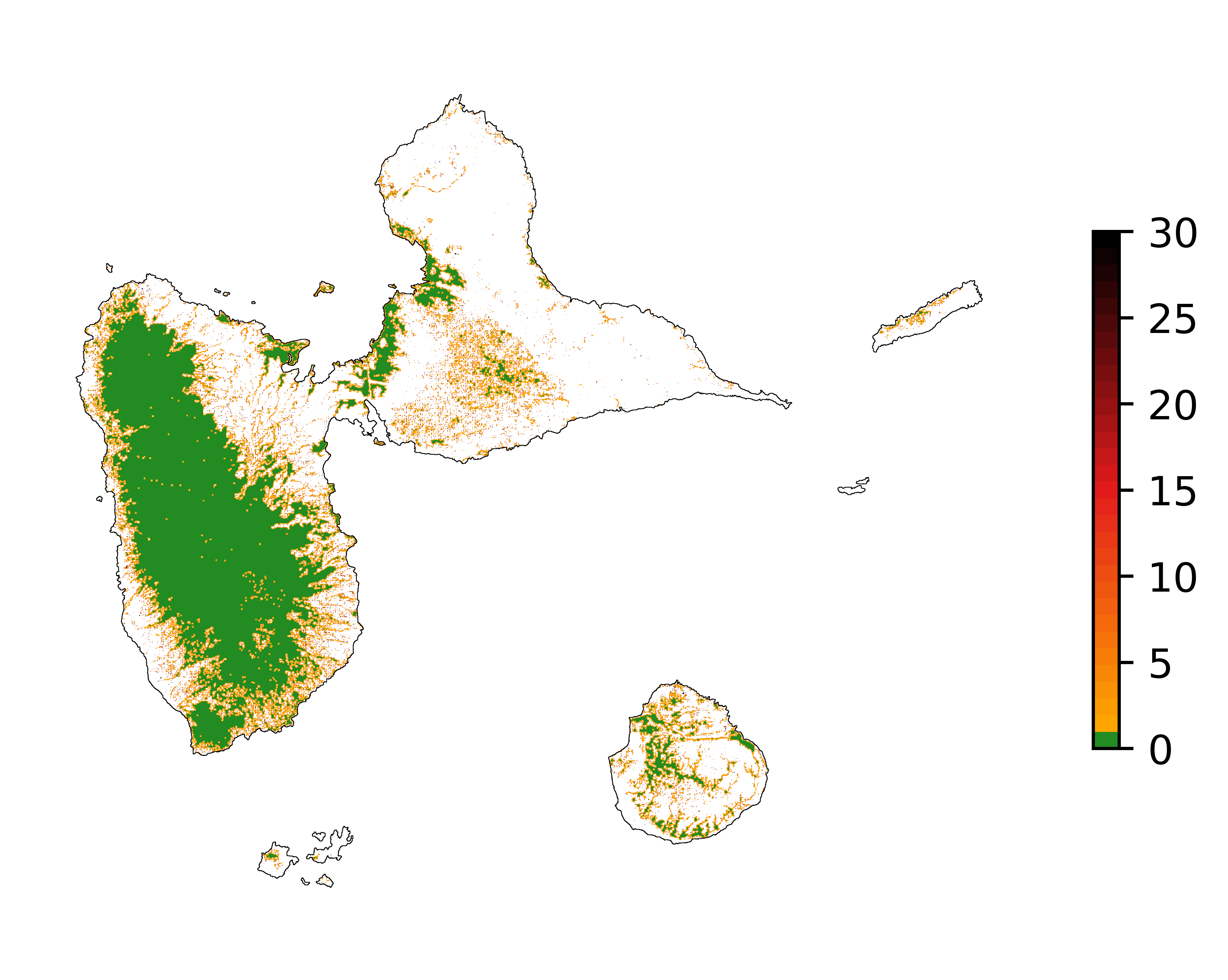
Map of the deforestation risk following the JNR methodology. Forest pixels are categorized in up to 30 classes of deforestation risk. Forest pixels which belong to the class 0 (in green) are located farther than a distance of 120 m from the forest edge and have a negligible risk of being deforested.
6 Deforestation rates per category of risk
Before the validation step, we need to compute the historical deforestation rates (in %/yr) for each category of spatial deforestation risk. The historical deforestation rates are computed for the calibration period (here 2000–2010). Deforestation rates provide estimates of the percentage of forest (which is then converted to an area of forest) that should be deforested inside each forest pixel which belongs to a given category of deforestation risk.
rmj.defrate_per_cat(
    fcc_file=fcc_file,
    defor_values=1,
    riskmap_file=os.path.join(out_dir, "riskmap.tif"),
    time_interval=10,
    tab_file_defrate=os.path.join(out_dir, "defrate_per_cat.csv"),
    blk_rows=128,
    verbose=False)
A table indicating the deforestation rate per category of deforestation is produced:
cat |
nfor |
ndefor |
rate |
|---|---|---|---|
1 |
361904 |
7766 |
0.002166880478294053 |
2 |
12770 |
5856 |
0.0595107240968078 |
3 |
6490 |
4379 |
0.10623292135671092 |
4 |
3119 |
2543 |
0.15542015960877786 |
5 |
1492 |
1342 |
0.20524687620953053 |
6 |
840 |
789 |
0.24433538025668888 |
7 |
476 |
457 |
0.2753727450970095 |
8 |
168 |
166 |
0.35794523801272426 |
9 |
12 |
12 |
1.0 |
10 |
0 |
0 |
|
11 |
0 |
0 |
|
12 |
0 |
0 |
|
13 |
0 |
0 |
|
14 |
0 |
0 |
|
15 |
0 |
0 |
|
16 |
0 |
0 |
|
17 |
0 |
0 |
|
18 |
0 |
0 |
|
19 |
0 |
0 |
|
20 |
0 |
0 |
|
21 |
0 |
0 |
|
22 |
0 |
0 |
|
23 |
0 |
0 |
|
24 |
0 |
0 |
|
25 |
0 |
0 |
|
26 |
0 |
0 |
|
27 |
0 |
0 |
|
28 |
0 |
0 |
|
29 |
0 |
0 |
|
30 |
6304 |
6304 |
1.0 |
From this table, we see that the deforestation rate increases with the deforestation risk category and that deforestation rates are spread on the interval [0, 1], suggesting that category 1 represents well a category with very low deforestation risk (close to 0), and category 30 represents well a category with very high deforestation risk (close to 1).
7 Derive a risk map at the beginning of the validation period
To derive the risk map at the beginning of the validation period, we consider (i) the forest cover at this date, (ii) the map of local deforestation rates, (ii) the threshold distance, and (iii) the bins used to categorize the deforestation rates. All these data are obtained from previous steps and based on the deforestation for the historical period. The approach is the following: first, we identify the forest pixels at the beginning of the validation period. Second, we assign category zero to pixels at a distance from the forest edge which is greater than the distance threshold. Third, we categorize the deforestation rates using the previous bins identified for the historical period. In addition to the risk map, two additional raster files are produced: the raster file of the distance to forest edge at the beginning of the validation period, and the raster file of local deforestation rates including the zero deforestation risk.
7.1 Distance to forest edge at the beginning of the validation period
rmj.dist_values(input_file=fcc_file,
                dist_file=os.path.join(out_dir, "dist_edge_v.tif"),
                values="0,1",
                verbose=False)
7.2 Raster of local deforestation rate at the beginning of the validation period
rmj.get_ldefz_v(
    ldefrate_file=os.path.join(out_dir, "ldefrate.tif"),
    dist_v_file=os.path.join(out_dir, "dist_edge_v.tif"),
    dist_thresh=120,
    ldefrate_with_zero_v_file=os.path.join(out_dir, "ldefrate_with_zero_v.tif"),
    blk_rows=128,
    verbose=False)
7.3 Risk map at the beginning of the validation period
rmj.get_riskmap_v(
    ldefrate_with_zero_v_file=os.path.join(out_dir, "ldefrate_with_zero_v.tif"),
    bins=bins,
    riskmap_v_file=os.path.join(out_dir, "riskmap_v.tif"),
    blk_rows=128,
    verbose=False)
8 Validation
The fifth step focuses on comparing the map of deforestation risk with a deforestation map corresponding to the validation period. The validation period follows the calibration period and provides independent observations of deforestation.
To do so, we consider a square grid of at least 1000 spatial cells containing at least one forest pixel at the beginning of the validation period. Following JNR specification, the cell size should be \(\leq\) 10 km. Note that with the map of deforestation risk, each forest pixel at the beginning of the validation period falls into a category of deforestation risk. For each cell of the grid, we compute the predicted area of deforestation (in ha) given the map of deforestation risk and the historical deforestation rates for each category of deforestation risk computed on the calibration period (see previous step).
We can then compare the predicted deforestation with the observed deforestation in that spatial cell for the validation period. Because all cells don’t have the same forest cover at the beginning of the validation period, a weight \(w_j\) is computed for each grid cell \(j\) such that \(w_j=\beta_j / B\), with \(\beta_j\) the forest cover (in ha) in the cell \(j\) at the beginning of the validation period and \(B\) the total forest cover in the jurisdiction (in ha) at the same date. We then calculate the weighted root mean squared error (wRMSE) from the observed and predicted deforestation for each cell and the cell weights.
We set the argument no_quantity_error to True to correct the total deforestation for the predictions and avoid a “quantity” error (sensu Pontius) due to the difference in total deforestation between periods. This is currently being discussed for improving the JNR methodology.
ofile = os.path.join(out_dir, "pred_obs.png")
rmj.validation(
    fcc_file=fcc_file,
    time_interval=10,
    riskmap_file=os.path.join(out_dir, "riskmap_v.tif"),
    tab_file_defrate=os.path.join(out_dir, "defrate_per_cat.csv"),
    csize=40,
    no_quantity_error=True,
    tab_file_pred=os.path.join(out_dir, "pred_obs.csv"),
    fig_file_pred=ofile,
    figsize=(6.4, 4.8),
    dpi=100, verbose=False)
ofile
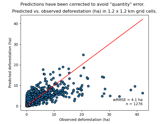
Relationship between observed and predicted deforestation in 1 x 1 km grid cells. The red line is the identity line. Values of the weighted root mean squared error (wRMSE, in ha) and of the number of observations (\(n\), the number of spatial cells) are reported on the graph.
9 Final risk map
The user must repeat the procedure and obtain risk maps for various window size and slicing algorithms. Following the JNR methodology, at least 25 different sizes for the moving window must be tested together with two slicing algorithms (“Equal Interval” and “Equal Area”), thus leading to a minimum of 50 different maps of deforestation risk. The map with the smallest wRMSE value is considered the best risk map. Once the best risk map is identified, with the corresponding window size and slicing algorithm, a final risk map is derived considering both the calibration and validation period (see the Get Started tutorial).