Kenya

1 Preamble

1.1 Importing Python modules

Import the Python modules needed to run the analysis.

# Imports
import os
import multiprocessing as mp
import pkg_resources
import time

import numpy as np
import pandas as pd
from tabulate import tabulate

import riskmapjnr as rmj

Increase the cache for GDAL to increase computational speed.

# GDAL
os.environ["GDAL_CACHEMAX"] = "1024"

Set the PROJ_LIB environmental variable.

os.environ["PROJ_LIB"] = "/home/ghislain/.pyenv/versions/miniconda3-latest/envs/conda-rmj/share/proj"

Create a directory to save results.

out_dir = "outputs_kenya"
rmj.make_dir(out_dir)

1.2 Forest cover change data

We consider recent forest cover change data for Kenya. The raster file (fcc123_KEN_101418.tif) includes the following values: 1 for deforestation on the period 2010–2014, 2 for deforestation on the period 2014–2018, and 3 for the remaining forest in 2018. NoData value is set to 0. The first period (2010–2014) will be used for calibration and the second period (2014–2018) will be used for validation.

fcc_file = "data/fcc123_KEN_101418.tif"
print(fcc_file)
border_file = "data/ctry_border_KEN.gpkg"
print(border_file)

data/fcc123_KEN_101418.tif
data/ctry_border_KEN.gpkg

We plot the forest cover change map with the plot.fcc123() function.

ofile = os.path.join(out_dir, "fcc123.png")
fig_fcc123 = rmj.plot.fcc123(
    input_fcc_raster=fcc_file,
    maxpixels=1e8,
    output_file=ofile,
    borders=border_file,
    linewidth=0.2,
    figsize=(5, 4), dpi=800)
ofile

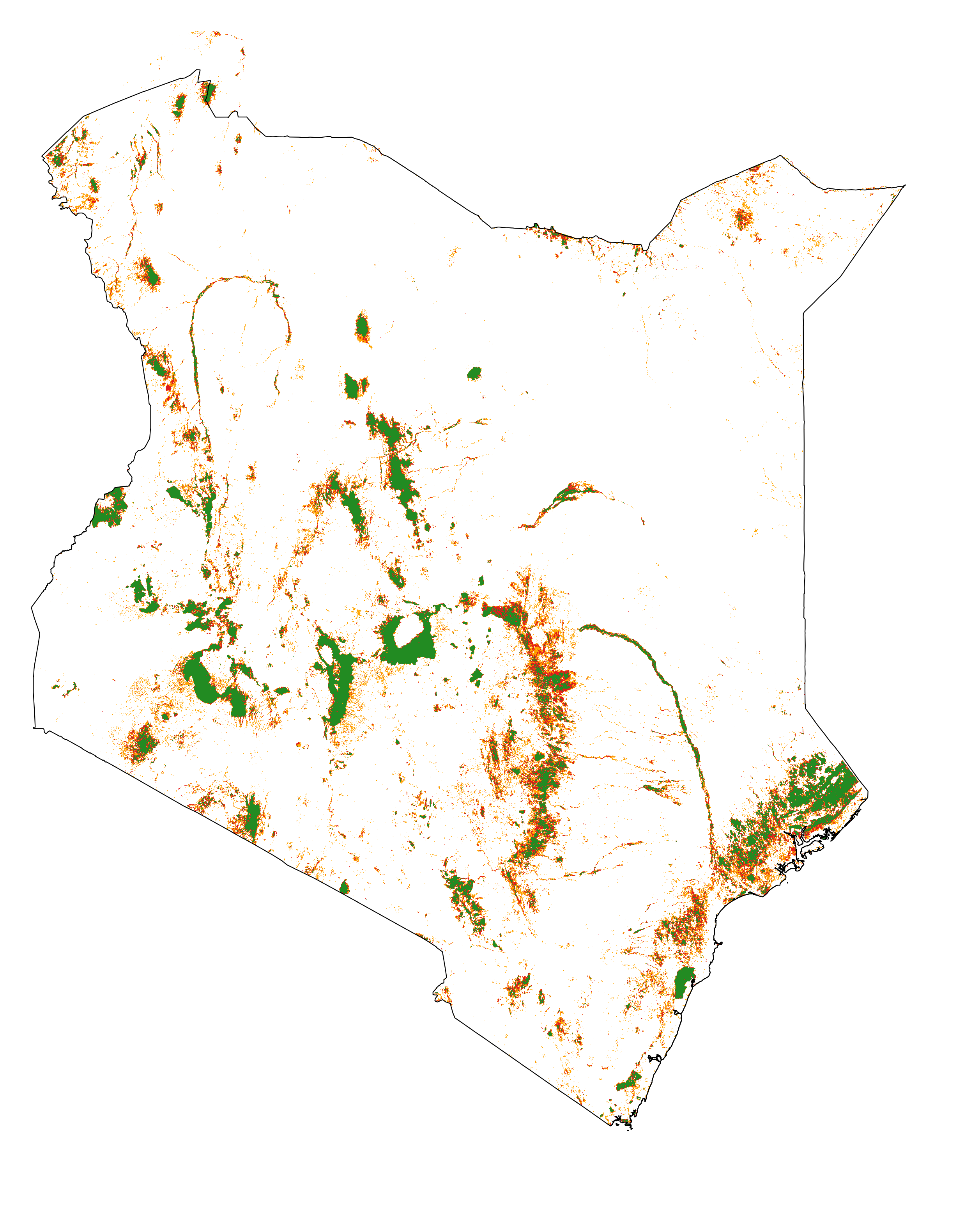
Forest cover change map. Deforestation on the first period (2010–2014) is in orange, deforestation on the second period (2014–2018) is in red and remaining forest (in 2018) is in green.

2 Deriving the deforestation risk map

We derive the deforestation risk map using the makemap() function. This function calls a sequence of functions from the riskmapjnr package which perform all the steps detailed in the JNR methodology. We can use parallel computing using several CPUs.

ncpu = mp.cpu_count() - 2
print(f"Number of CPUs: {ncpu}.")

Number of CPUs: 6.

start_time = time.time()
results_makemap = rmj.makemap(
    fcc_file=fcc_file,
    time_interval=[4, 4],
    output_dir=out_dir,
    clean=False,
    dist_bins=np.arange(0, 1080, step=30),
    win_sizes=np.arange(5, 200, 16),
    ncat=30,
    parallel=True,
    ncpu=ncpu,
    methods=["Equal Interval", "Equal Area"],
    csize=400,  # 12 km
    no_quantity_error=True,
    figsize=(6.4, 4.8),
    dpi=100,
    blk_rows=200,
    verbose=True)
sec_seq = time.time() - start_time

print('Computation time:', time.strftime("%H:%M:%S",time.gmtime(sec_seq)))

Computation time: 00:49:43

3 Results

3.1 Deforestation risk and distance to forest edge

We obtain the threshold for the distance to forest edge beyond which the deforestation risk is negligible.

dist_thresh = results_makemap["dist_thresh"]
print(f"The distance theshold is {dist_thresh} m.")

The distance theshold is 780 m.

We have access to a table indicating the cumulative percentage of deforestation as a function of the distance to forest edge.

Distance	Npixels	Area	Cumulation	Percentage
30	1.4005e+07	1.26045e+06	1.26045e+06	48.9547
60	5.35311e+06	481780	1.74223e+06	67.6666
90	3.02736e+06	272463	2.01469e+06	78.2489
120	1.49449e+06	134504	2.1492e+06	83.4729
150	1.17144e+06	105430	2.25463e+06	87.5677
180	639743	57576.9	2.3122e+06	89.8039
210	469736	42276.2	2.35448e+06	91.4459
240	417499	37574.9	2.39205e+06	92.9053
270	326224	29360.2	2.42141e+06	94.0456
300	260730	23465.7	2.44488e+06	94.957
330	179341	16140.7	2.46102e+06	95.5839
360	147688	13291.9	2.47431e+06	96.1001
390	153559	13820.3	2.48813e+06	96.6369
420	109451	9850.59	2.49798e+06	97.0195
450	98440	8859.6	2.50684e+06	97.3636
480	72145	6493.05	2.51334e+06	97.6158
510	70682	6361.38	2.5197e+06	97.8628
540	58834	5295.06	2.52499e+06	98.0685
570	53707	4833.63	2.52983e+06	98.2562
600	47735	4296.15	2.53412e+06	98.4231
630	36436	3279.24	2.5374e+06	98.5504
660	38346	3451.14	2.54085e+06	98.6845
690	30219	2719.71	2.54357e+06	98.7901
720	26853	2416.77	2.54599e+06	98.884
750	27575	2481.75	2.54847e+06	98.9804
780	22398	2015.82	2.55049e+06	99.0586
810	20402	1836.18	2.55232e+06	99.13
840	17439	1569.51	2.55389e+06	99.1909
870	16532	1487.88	2.55538e+06	99.2487
900	17080	1537.2	2.55692e+06	99.3084

We also have access to a plot showing how the cumulative percentage of deforestation increases with the distance to forest edge.

os.path.join(out_dir, "fullhist/perc_dist.png")

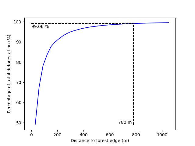
Identifying areas for which the risk of deforestation is negligible. Figure shows that more than 99% of the deforestation occurs within a distance from the forest edge ≤ 180 m. Forest areas located at a distance > 180 m from the forest edge can be considered as having no risk of being deforested.

3.2 Model comparison

We can plot the change in wRMSE value with both the window size and slicing algorithm. It seems that the “Equal Interval” (ei) algorithm provides lower wRMSE values. The lowest wRMSE value is obtained for a window size between 25 and 50 pixels.

os.path.join(out_dir, "modcomp/mod_comp.png")

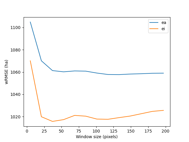
Change in wRMSE values as a function of both window size and slicing algorithm. “ei” is the “Equal Interval” algorithm and “ea” is the “Equal Area” algorithm.

We identify the moving window size and the slicing algorithm of the best model.

ws_hat = results_makemap["ws_hat"]
m_hat = results_makemap["m_hat"]
print(f"The best moving window size is {ws_hat} pixels.")
print(f"The best slicing algorithm is '{m_hat}'.")

The best moving window size is 37 pixels.
The best slicing algorithm is 'ei'.

3.3 Model performance

We can look at the relationship between observed and predicted deforestation in 1 x 1 km grid cells for the best model.

os.path.join(out_dir, f"modcomp/pred_obs_ws{ws_hat}_{m_hat}.png")

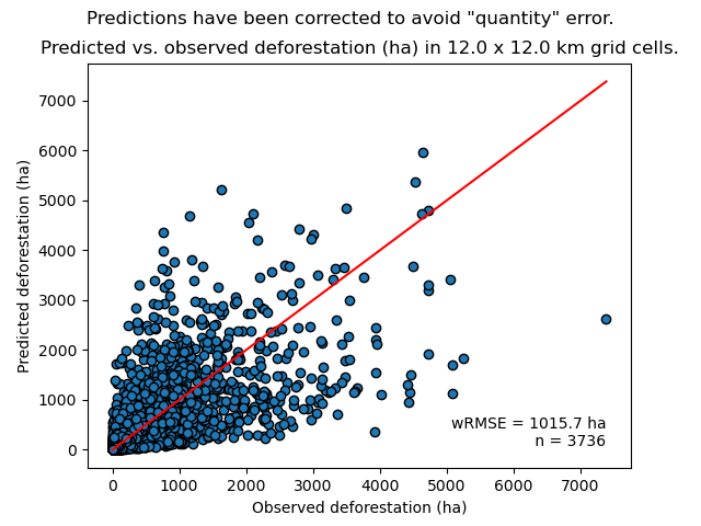
Relationship between observed and predicted deforestation in 1 x 1 km grid cells for the best model. The red line is the identity line. Values of the weighted root mean squared error (wRMSE, in ha) and of the number of observations (\(n\), the number of spatial cells) are reported on the graph.

3.4 Risk map of deforestation

We plot the risk map using the plot.riskmap() function.

ifile = os.path.join(out_dir, f"endval/riskmap_ws{ws_hat}_{m_hat}_ev.tif")
ofile = os.path.join(out_dir, f"endval/riskmap_ws{ws_hat}_{m_hat}_ev.png")
riskmap_fig = rmj.plot.riskmap(
    input_risk_map=ifile,
    maxpixels=1e8,
    output_file=ofile,
    borders=border_file,
    legend=True,
    figsize=(5, 4), dpi=800, linewidth=0.2,)
ofile

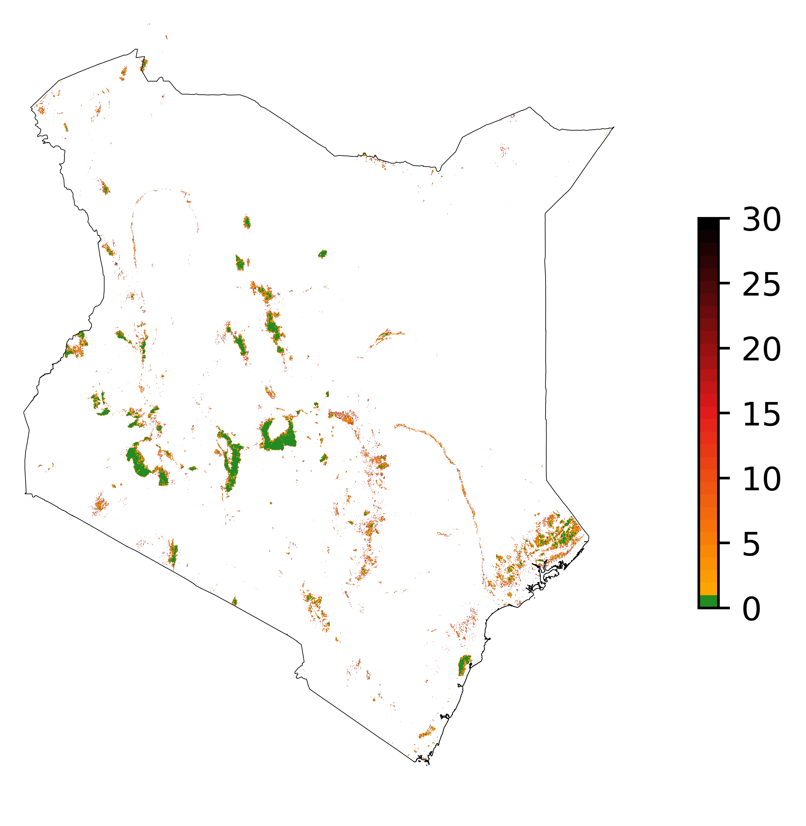
Map of the deforestation risk following the JNR methodology. Forest pixels are categorized in up to 30 classes of deforestation risk. Forest pixels which belong to the class 0 (in green) are located farther than a distance of 780 m from the forest edge and have a negligible risk of being deforested.