Species distribution models (SDM) are useful tools to explain or predict species range and abundance from various environmental factors. SDM are thus widely used in conservation biology. When using field observations (occurence or abundance data) to fit SDMs, two major problems can arise leading to potential bias in models’ results: imperfect detection (Lahoz-Monfort, Guillera-Arroita & Wintle 2014) and spatial dependence of the observations (Lichstein et al. 2002). In this vignette, we illustrate the use of the hSDM R package wich aims at providing user-friendly statistical functions to account for both imperfect detection and spatial dependence. Package’s functions are developped in a hierarchical Bayesian framework. Functions call a Metropolis-within-Gibbs algorithm coded in C to estimate model’s parameters. Using compiled C code for the Gibbs sampler reduce drastically the computation time. By making these new statistical tools available to the scientific community, we hope to democratize the use of more complex, but more realistic, statistical models for increasing knowledge in ecology and conserving biodiversity.
Below, we show an example of the use of hSDM for fitting a species distribution model to abundance data for a bird species. Model types available in hSDM are not limited to those described in this example. hSDM includes various model types (for various contexts: imperfect detection, spatial dependence, zero-inflation, land transformation) for both occurrence and abundance data:
- simple Binomial and Poisson models (Clark 2007)
- site-occupancy models (MacKenzie et al. 2002)
- N-mixture models (Royle 2004)
- Zero-Inflated Binomial (ZIB) models (Wilson & Jetz 2016)
- Zero-Inflated Poisson (ZIP) models (Flores, Rossi & Mortier 2009)
- less common mixture models to account for land degradation (Latimer et al. 2006)
All the above models can include an additional intrinsic conditional autoregressive (iCAR) process to account for the spatial dependence of the observations. It should be easy for the user to fit other model types from the example below as function arguments are rather similar from one model to the other.
1 Data-set
The data-set from Kéry & Andrew Royle (2010) includes repeated count data for the Willow tit (Poecile montanus, a pesserine bird, Fig. 1.1) in Switzerland on the period 1999-2003. Data come from the Swiss national breeding bird survey MHB (Monitoring Haüfige Brutvögel). MHB is based on 264 1-km\(^2\) sampling units (quadrats) laid out as a grid (Fig. 1.2). Since 1999, every quadrat has been surveyed two to three times during most breeding seasons (15 April to 15 July). The Willow tit is a widespread but moderately rare bird species. It has a weak song and elusive behaviour and can be rather difficult to detect.

Figure 1.1: Willow tit (Poecile montanus).
We first load some necessary packages. The sp and raster packages will be used for manipulating spatial data.
# Load libraries
library(sp)
#> The legacy packages maptools, rgdal, and rgeos, underpinning the sp package,
#> which was just loaded, will retire in October 2023.
#> Please refer to R-spatial evolution reports for details, especially
#> https://r-spatial.org/r/2023/05/15/evolution4.html.
#> It may be desirable to make the sf package available;
#> package maintainers should consider adding sf to Suggests:.
#> The sp package is now running under evolution status 2
#>      (status 2 uses the sf package in place of rgdal)
library(raster)
library(hSDM)
#> ##
#> ## hSDM R package
#> ## For hierarchical Bayesian species distribution models
#> ##
This data-set from Kéry & Andrew Royle (2010) is available in the hSDM R package. It can be loaded with the data command and formated to be used with hSDM functions. The data is in “wide” format: each line is a site and the repeated count data (from count1 to count3) are in columns. A site is characterized by its x-y geographical coordinates, elevation (in m) and forest cover (in %). The date of each observation (julian date) has been recorded.
# Load Kéry et al. 2010 data
data(data.Kery2010, package="hSDM")
head(data.Kery2010)
#>   coordx coordy elevation forest count1 count2 count3 juldate1 juldate2
#> 1    497    118       450      3      0      0      0      114      139
#> 2    503    134       450     21      0      0      0      108      130
#> 3    503    158      1050     32      1      1      0      116      145
#> 4    509    166      1150     35      0      0      0      106      134
#> 5    509    150       950     NA      0      0      0      121      152
#> 6    521    150       550      2      0      0      0      114      141
#>   juldate3
#> 1      166
#> 2      158
#> 3      177
#> 4      160
#> 5      166
#> 6      150
We first normalize the data to facilitate MCMC convergence. We discard the forest cover in our example.
# Normalized variables
elev.mean <- mean(data.Kery2010$elevation)
elev.sd <- sd(data.Kery2010$elevation)
juldate.mean <- mean(c(data.Kery2010$juldate1,
                     data.Kery2010$juldate2,
                     data.Kery2010$juldate3),na.rm=TRUE)
juldate.sd <- sd(c(data.Kery2010$juldate1,
                 data.Kery2010$juldate2,
                 data.Kery2010$juldate3),na.rm=TRUE)
data.Kery2010$elevation <- (data.Kery2010$elevation-elev.mean)/elev.sd
data.Kery2010$juldate1 <- (data.Kery2010$juldate1-juldate.mean)/juldate.sd
data.Kery2010$juldate2 <- (data.Kery2010$juldate2-juldate.mean)/juldate.sd
data.Kery2010$juldate3 <- (data.Kery2010$juldate3-juldate.mean)/juldate.sd
We plot the observation sites over a grid of 10 \(\times\) 10 km\(^2\) cells.
# Landscape and observation sites
sites.sp <- SpatialPointsDataFrame(coords=data.Kery2010[c("coordx","coordy")],
                                   data=data.Kery2010[,-c(1,2)])
xmin <- min(data.Kery2010$coordx)
xmax <- max(data.Kery2010$coordx)
ymin <- min(data.Kery2010$coordy)
ymax <- max(data.Kery2010$coordy)
res_spatial_cell <- 10
ncol <- ceiling((xmax-xmin)/res_spatial_cell)
nrow <- ceiling((ymax-ymin)/res_spatial_cell)
Xmax <- xmin+ncol*res_spatial_cell
Ymax <- ymin+nrow*res_spatial_cell
ext <- extent(c(xmin, Xmax,
                ymin, Ymax))
landscape <- raster(ncols=ncol,nrows=nrow,ext)
values(landscape) <- runif(ncell(landscape),0,1)
landscape.po <- rasterToPolygons(landscape)
par(mar=c(0.1,0.1,0.1,0.1))
plot(landscape.po)
points(sites.sp, pch=16, cex=1, col="black")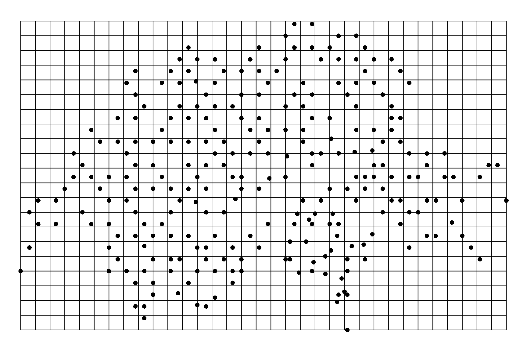
Figure 1.2: Location of the 264 10 km\(^2\) quadrats of the Swiss national breeding bird survey. Points are located on a grid of 10 km\(^2\) cells. The grid is covering the geographical extent of the observation points.
One important step if we want to account for spatial dependence is to compute the neighborhood for each cell. In our case, the neighborhood is define by the “king move” in chess, in the height directions around the target cell. To compute the neighbordhood for each cell, we need the number of neighbors (which can vary) and the adjacent cell identifiers. We can use the function adjacent from the raster package to do this.
# Neighborhood
# Rasters must be projected to correctly compute the neighborhood
crs(landscape) <- '+proj=utm +zone=1'
#> Warning in sp::CRS(...): sf required for evolution_status==2L
# Cell for each site
cells <- extract(landscape,sites.sp,cell=TRUE)[,1]
# Neighborhood matrix
ncells <- ncell(landscape)
neighbors.mat <- adjacent(landscape, cells=c(1:ncells), directions=8,
                          pairs=TRUE, sorted=TRUE)
# Number of neighbors by cell
n.neighbors <- as.data.frame(table(as.factor(neighbors.mat[,1])))[,2]
# Adjacent cells
adj <- neighbors.mat[,2]
We rearrange the data in two data-sets, one for the observation (or detection) process and one for the suitability (or ecological) process. The data for the observation process is in “long” format. Each row is an observation which is characterized by the site number and the julian date of the observation. The data for the suitability process (at the site level) includes information on sites (coordinates and elevation) by row.
# Arranging data
# data.obs
nsite <- length(data.Kery2010$coordx)
count <- c(data.Kery2010$count1,data.Kery2010$count2,data.Kery2010$count3)
juldate <- c(data.Kery2010$juldate1,data.Kery2010$juldate2,
             data.Kery2010$juldate3)
site <- rep(1:nsite,3)
data.obs <- data.frame(count,juldate,site)
data.obs <- data.obs[!is.na(data.obs$juldate),]
# data.suit
data.suit <- data.Kery2010[c("coordx","coordy","elevation")]
data.suit$cells <- cells
data.suit <- data.suit[-139,] # Removing site 139 with no juldate
We will compare three SDMs with increasing complexity: a first simple Poisson model, a second N-mixture model with imperfect detection, and a third N-mixture iCAR model with imperfect detection and spatial dependence.
2 Simple Poisson model
To fit a simple Poisson model, we use the function hSDM.poisson. For this model, we slightly rearrange the observation data-set to associate the site altitude to each observation in a “long” format. The statistical model can be written as follow:
\[\begin{equation} y_i \sim \mathcal{P}oisson(\lambda_i) \\ \log(\lambda_i) = X_i \beta \\ \end{equation}\]
# hSDM.poisson
data.pois <- data.obs
data.pois$elevation <- data.suit$elevation[as.numeric(as.factor(data.obs$site))]
mod.Kery2010.pois <- hSDM.poisson(counts=data.pois$count,
                                  suitability=~elevation+I(elevation^2),
                                  data=data.pois, beta.start=0)
#>
#> Running the Gibbs sampler. It may be long, please keep cool :)
#>
#> **********:10.0%, mean accept. rates= beta:0.473
#> **********:20.0%, mean accept. rates= beta:0.437
#> **********:30.0%, mean accept. rates= beta:0.460
#> **********:40.0%, mean accept. rates= beta:0.430
#> **********:50.0%, mean accept. rates= beta:0.430
#> **********:60.0%, mean accept. rates= beta:0.443
#> **********:70.0%, mean accept. rates= beta:0.470
#> **********:80.0%, mean accept. rates= beta:0.443
#> **********:90.0%, mean accept. rates= beta:0.413
#> **********:100.0%, mean accept. rates= beta:0.463
# Outputs
summary(mod.Kery2010.pois$mcmc)
#>
#> Iterations = 5001:14991
#> Thinning interval = 10
#> Number of chains = 1
#> Sample size per chain = 1000
#>
#> 1. Empirical mean and standard deviation for each variable,
#>    plus standard error of the mean:
#>
#>                           Mean      SD Naive SE Time-series SE
#> beta.(Intercept)       0.02908 0.06369 0.002014       0.003676
#> beta.elevation         3.07617 0.16616 0.005254       0.018741
#> beta.I(elevation^2)   -1.79461 0.11144 0.003524       0.011860
#> Deviance            2157.97699 2.35949 0.074614       0.137429
#>
#> 2. Quantiles for each variable:
#>
#>                           2.5%        25%        50%       75%     97.5%
#> beta.(Intercept)      -0.09654   -0.01742    0.02864    0.0744    0.1528
#> beta.elevation         2.76477    2.95534    3.07390    3.1958    3.3890
#> beta.I(elevation^2)   -2.02038   -1.87021   -1.79278   -1.7178   -1.5802
#> Deviance            2155.19872 2156.26439 2157.38672 2159.0371 2164.2946
# Predictions
npred <- 100
nsamp <- dim(mod.Kery2010.pois$mcmc)[1]
# Abundance-elevation
elev.seq <- seq(500,3000,length.out=npred)
elev.seq.n <- (elev.seq-elev.mean)/elev.sd
beta <- as.matrix(mod.Kery2010.pois$mcmc[,1:3])
tbeta <- t(beta)
X <- matrix(c(rep(1,npred),elev.seq.n,elev.seq.n^2),ncol=3)
N <- matrix(NA,nrow=nsamp,ncol=npred)
for (i in 1:npred) {
    N[,i] <- exp(X[i,] %*% tbeta)
}
N.est.pois <- apply(N,2,mean)
N.q1.pois <- apply(N,2,quantile,0.025)
N.q2.pois <- apply(N,2,quantile,0.975)
3 N-mixture model for imperfect detection
The model integrates two processes, an ecological process associated to the abundance of the species due to habitat suitability and an observation process that takes into account the fact that the probability of detection of the species is inferior to one.
\[\begin{equation} \textbf{Ecological process:} \\ N_i \sim \mathcal{P}oisson(\lambda_i) \\ \log(\lambda_i) = X_i \beta \\ ~ \\ \textbf{Observation process:} \\ y_{it} \sim \mathcal{B}inomial(N_i, \delta_{it}) \\ \text{logit}(\delta_{it}) = W_{it} \gamma \\ \end{equation}\]
# hSDM.Nmixture
mod.Kery2010.Nmix <- hSDM.Nmixture(# Observations
                     counts=data.obs$count,
                     observability=~juldate+I(juldate^2),
                     site=data.obs$site,
                     data.observability=data.obs,
                     # Habitat
                     suitability=~elevation+I(elevation^2),
                     data.suitability=data.suit,
                     # Predictions
                     suitability.pred=NULL,
                     # Chains
                     burnin=10000, mcmc=5000, thin=5,
                     # Starting values
                     beta.start=0,
                     gamma.start=0,
                     # Priors
                     mubeta=0, Vbeta=1.0E6,
                     mugamma=0, Vgamma=1.0E6,
                     # Various
                     seed=1234, verbose=1,
                     save.p=0, save.N=0)
#>
#> Running the Gibbs sampler. It may be long, please keep cool :)
#>
#> **********:10.0%, mean accept. rates= beta:0.213, gamma:0.253, N:0.172
#> **********:20.0%, mean accept. rates= beta:0.240, gamma:0.230, N:0.205
#> **********:30.0%, mean accept. rates= beta:0.240, gamma:0.247, N:0.183
#> **********:40.0%, mean accept. rates= beta:0.270, gamma:0.250, N:0.193
#> **********:50.0%, mean accept. rates= beta:0.327, gamma:0.233, N:0.189
#> **********:60.0%, mean accept. rates= beta:0.313, gamma:0.263, N:0.197
#> **********:70.0%, mean accept. rates= beta:0.273, gamma:0.223, N:0.211
#> **********:80.0%, mean accept. rates= beta:0.257, gamma:0.240, N:0.218
#> **********:90.0%, mean accept. rates= beta:0.310, gamma:0.300, N:0.168
#> **********:100.0%, mean accept. rates= beta:0.257, gamma:0.230, N:0.206
# Outputs
summary(mod.Kery2010.Nmix$mcmc)
#>
#> Iterations = 10001:14996
#> Thinning interval = 5
#> Number of chains = 1
#> Sample size per chain = 1000
#>
#> 1. Empirical mean and standard deviation for each variable,
#>    plus standard error of the mean:
#>
#>                          Mean       SD Naive SE Time-series SE
#> beta.(Intercept)       0.6484  0.08698 0.002750       0.007622
#> beta.elevation         2.9294  0.20188 0.006384       0.031113
#> beta.I(elevation^2)   -1.8782  0.13632 0.004311       0.019594
#> gamma.(Intercept)      0.2419  0.10853 0.003432       0.009402
#> gamma.juldate         -0.2356  0.08556 0.002706       0.004650
#> gamma.I(juldate^2)     0.2705  0.08694 0.002749       0.006721
#> Deviance            1889.7198 29.49971 0.932863       2.417696
#>
#> 2. Quantiles for each variable:
#>
#>                           2.5%       25%       50%       75%      97.5%
#> beta.(Intercept)       0.47179    0.5895    0.6484    0.7112    0.80779
#> beta.elevation         2.52078    2.7878    2.9250    3.0673    3.30330
#> beta.I(elevation^2)   -2.14580   -1.9673   -1.8808   -1.7859   -1.59867
#> gamma.(Intercept)      0.02988    0.1652    0.2435    0.3228    0.45101
#> gamma.juldate         -0.41117   -0.2907   -0.2347   -0.1766   -0.07425
#> gamma.I(juldate^2)     0.10274    0.2137    0.2704    0.3317    0.43780
#> Deviance            1837.06422 1868.9839 1887.4536 1907.9318 1954.82932
# Predictions
nsamp <- dim(mod.Kery2010.Nmix$mcmc)[1]
# Abundance-elevation
beta <- as.matrix(mod.Kery2010.Nmix$mcmc[,1:3])
tbeta <- t(beta)
N <- matrix(NA,nrow=nsamp,ncol=npred)
for (i in 1:npred) {
    N[,i] <- exp(X[i,] %*% tbeta)
}
N.est.Nmix <- apply(N,2,mean)
N.q1.Nmix <- apply(N,2,quantile,0.025)
N.q2.Nmix <- apply(N,2,quantile,0.975)
# Detection-Julian date
juldate.seq <- seq(100,200,length.out=npred)
juldate.seq.n <- (juldate.seq-juldate.mean)/juldate.sd
gamma <- as.matrix(mod.Kery2010.Nmix$mcmc[,4:6])
tgamma <- t(gamma)
W <- matrix(c(rep(1,npred),juldate.seq.n,juldate.seq.n^2),ncol=3)
delta <- matrix(NA,nrow=nsamp,ncol=npred)
for (i in 1:npred) {
    delta[,i] <- inv.logit(X[i,] %*% tgamma)
}
delta.est.Nmix <- apply(delta,2,mean)
delta.q1.Nmix <- apply(delta,2,quantile,0.025)
delta.q2.Nmix <- apply(delta,2,quantile,0.975)
4 N-mixture model with iCAR process
For this model, we assume that the abundance of the species at one site depends on the abundance of the species on neighboring sites. In this model, the ecological process includes an intrinsic conditional autoregressive (iCAR) subprocess to model the spatial dependence between observations.
\[\begin{equation} \textbf{Ecological process:} \\ N_i \sim \mathcal{P}oisson(\lambda_i) \\ \log(\lambda_i) = X_i \beta + \rho_{j(i)} \\ \text{$\rho_{j(i)}$: spatial random effect for spatial entity $j$ including site $i$} \\ ~ \\ \textbf{Spatial dependence:} \\ \text{An intrinsic conditional autoregressive model (iCAR) is assumed:} \\ \rho_j \sim \mathcal{N}ormal(\mu_j, V_{\rho}/n_j) \\ \text{$\mu_j$: mean of $\rho_{j^{\prime}}$ in the neighborhood of $j$.} \\ \text{$V_{\rho}$: variance of the spatial random effects.} \\ \text{$n_j$: number of neighbors for spatial entity $j$.} \\ ~ \\ \textbf{Observation process:} \\ y_{it} \sim \mathcal{B}inomial(N_i, \delta_{it}) \\ \text{logit}(\delta_{it}) = W_{it} \gamma \\ \end{equation}\]
# hSDM.Nmixture.iCAR
mod.Kery2010.Nmix.iCAR <- hSDM.Nmixture.iCAR(# Observations
                            counts=data.obs$count,
                            observability=~juldate+I(juldate^2),
                            site=data.obs$site,
                            data.observability=data.obs,
                            # Habitat
                            suitability=~elevation+I(elevation^2),
                            data.suitability=data.suit,
                            # Spatial structure
                            spatial.entity=data.suit$cells,
                            n.neighbors=n.neighbors, neighbors=adj,
                            # Chains
                            burnin=20000, mcmc=10000, thin=10,
                            # Starting values
                            beta.start=0,
                            gamma.start=0,
                            Vrho.start=1,
                            # Priors
                            mubeta=0, Vbeta=1.0E6,
                            mugamma=0, Vgamma=1.0E6,
                            priorVrho="1/Gamma",
                            shape=1, rate=1,
                            # Various
                            seed=1234, verbose=1,
                            save.rho=0, save.p=0, save.N=0)
#>
#> Running the Gibbs sampler. It may be long, please keep cool :)
#>
#> **********:10.0%, mean accept. rates= beta:0.263, gamma:0.257, rho:0.257, N:0.279
#> **********:20.0%, mean accept. rates= beta:0.270, gamma:0.253, rho:0.250, N:0.232
#> **********:30.0%, mean accept. rates= beta:0.260, gamma:0.263, rho:0.283, N:0.251
#> **********:40.0%, mean accept. rates= beta:0.237, gamma:0.277, rho:0.253, N:0.249
#> **********:50.0%, mean accept. rates= beta:0.270, gamma:0.290, rho:0.252, N:0.232
#> **********:60.0%, mean accept. rates= beta:0.253, gamma:0.297, rho:0.280, N:0.234
#> **********:70.0%, mean accept. rates= beta:0.313, gamma:0.297, rho:0.254, N:0.285
#> **********:80.0%, mean accept. rates= beta:0.283, gamma:0.250, rho:0.281, N:0.279
#> **********:90.0%, mean accept. rates= beta:0.323, gamma:0.250, rho:0.289, N:0.236
#> **********:100.0%, mean accept. rates= beta:0.287, gamma:0.273, rho:0.275, N:0.248
summary(mod.Kery2010.Nmix.iCAR$mcmc)
#>
#> Iterations = 20001:29991
#> Thinning interval = 10
#> Number of chains = 1
#> Sample size per chain = 1000
#>
#> 1. Empirical mean and standard deviation for each variable,
#>    plus standard error of the mean:
#>
#>                          Mean       SD Naive SE Time-series SE
#> beta.(Intercept)       0.3749  0.32613 0.010313       0.040265
#> beta.elevation         1.9973  0.84697 0.026784       0.279847
#> beta.I(elevation^2)   -2.1986  0.48710 0.015403       0.142238
#> gamma.(Intercept)     -0.8790  0.20105 0.006358       0.062329
#> gamma.juldate         -0.1735  0.06543 0.002069       0.003898
#> gamma.I(juldate^2)     0.1589  0.05885 0.001861       0.004153
#> Vrho                  18.1555  4.97802 0.157419       0.547617
#> Deviance            1336.0869 48.14174 1.522376       9.021355
#>
#> 2. Quantiles for each variable:
#>
#>                           2.5%       25%       50%       75%      97.5%
#> beta.(Intercept)      -0.20728    0.1364    0.3661    0.6001    1.02133
#> beta.elevation         0.62581    1.2987    1.8709    2.6526    3.65104
#> beta.I(elevation^2)   -3.32975   -2.5131   -2.1079   -1.8235   -1.45366
#> gamma.(Intercept)     -1.29729   -1.0030   -0.8879   -0.7457   -0.48283
#> gamma.juldate         -0.29657   -0.2167   -0.1739   -0.1309   -0.04227
#> gamma.I(juldate^2)     0.04234    0.1187    0.1607    0.1958    0.27203
#> Vrho                  10.78215   14.6705   17.4504   20.7555   30.86624
#> Deviance            1248.61524 1302.4338 1334.8412 1368.8538 1430.86366
# Spatial random effects
rho.pred <- mod.Kery2010.Nmix.iCAR$rho.pred
r.rho.pred <- rasterFromXYZ(cbind(coordinates(landscape),rho.pred))
plot(r.rho.pred)
# Mean abundance by site
ma <- apply(sites.sp@data[,3:5],1,mean,na.rm=TRUE)
points(sites.sp,pch=16,cex=0.5)
points(sites.sp,pch=1,cex=ma/2)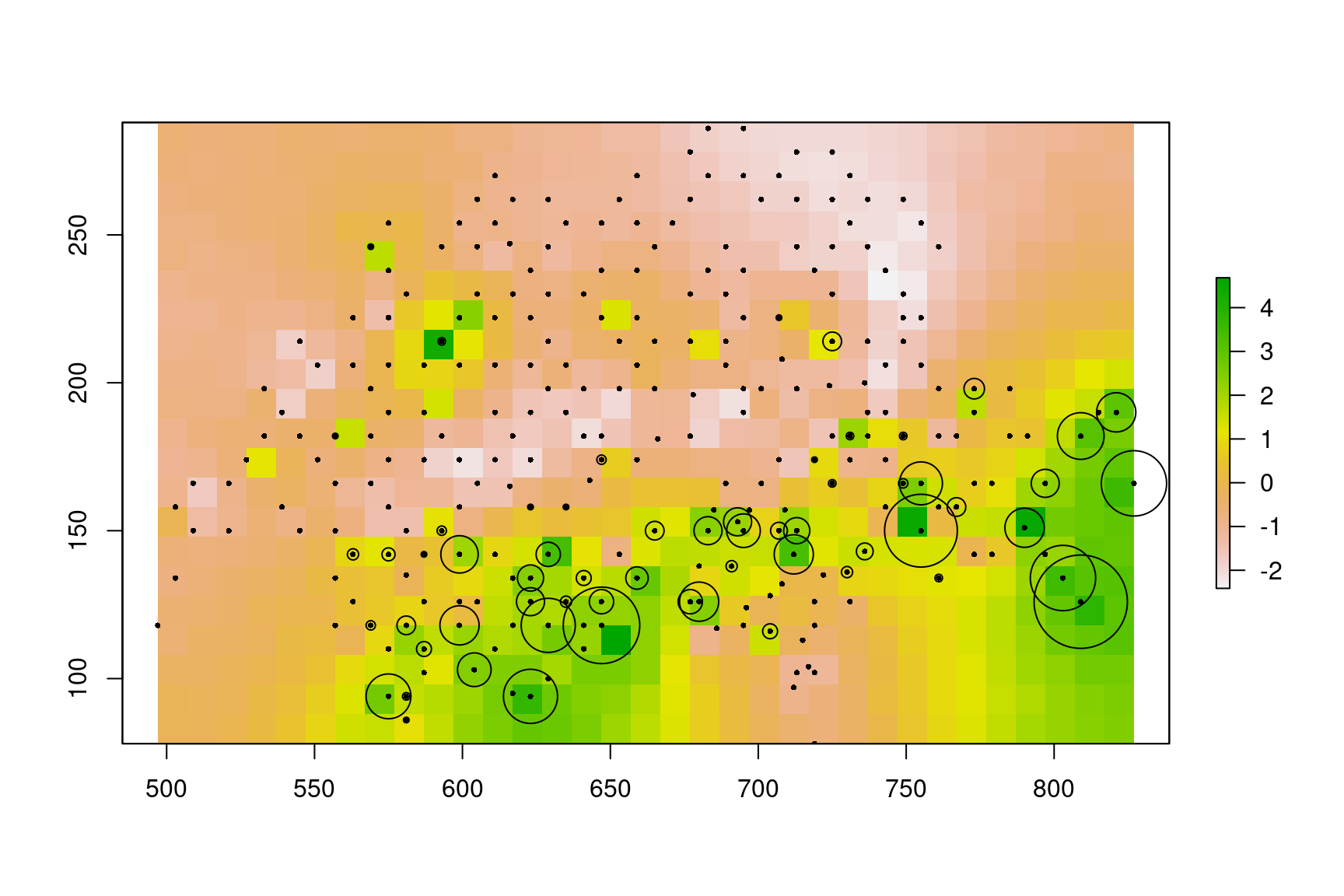
Figure 4.1: Estimated spatial random effects. Locations of observation quadrats are represented by dots. The mean abundance on each quadrat is represented by a circle of size proportional to abundance.
# Predictions
nsamp <- dim(mod.Kery2010.Nmix.iCAR$mcmc)[1]
# Abundance-elevation
beta <- as.matrix(mod.Kery2010.Nmix.iCAR$mcmc[,1:3])
tbeta <- t(beta)
N <- matrix(NA,nrow=nsamp,ncol=npred)
# Simplified way of obtaining samples for rho
rho.samp <- sample(rho.pred,nsamp,replace=TRUE)
for (i in 1:npred) {
    N[,i] <- exp(X[i,] %*% tbeta + rho.samp)
}
N.est.Nmix.iCAR <- apply(N,2,mean)
N.q1.Nmix.iCAR <- apply(N,2,quantile,0.025)
N.q2.Nmix.iCAR <- apply(N,2,quantile,0.975)

# Detection-Julian date
gamma <- as.matrix(mod.Kery2010.Nmix.iCAR$mcmc[,4:6])
tgamma <- t(gamma)
delta <- matrix(NA,nrow=nsamp,ncol=npred)
for (i in 1:npred) {
    delta[,i] <- inv.logit(X[i,] %*% tgamma)
}
delta.est.Nmix.iCAR <- apply(delta,2,mean)
delta.q1.Nmix.iCAR <- apply(delta,2,quantile,0.025)
delta.q2.Nmix.iCAR <- apply(delta,2,quantile,0.975)
5 Comparing predictions from the three different models
# Expected abundance - Elevation
par(mar=c(4,4,1,1),cex=1.4,tcl=+0.5)
plot(elev.seq,N.est.pois,type="l",
     xlim=c(500,3000),
     ylim=c(0,10),
     lwd=2,
     xlab="Elevation (m a.s.l.)",
     ylab="Expected abundance",
     axes=FALSE)
#lines(elev.seq,N.q1.pois,lty=3,lwd=1)
#lines(elev.seq,N.q2.pois,lty=3,lwd=1)
axis(1,at=seq(500,3000,by=500),labels=seq(500,3000,by=500))
axis(2,at=seq(0,10,by=2),labels=seq(0,10,by=2))
# Nmix
lines(elev.seq,N.est.Nmix,lwd=2,col="red")
#lines(elev.seq,N.q1.Nmix,lty=3,lwd=1,col="red")
#lines(elev.seq,N.q2.Nmix,lty=3,lwd=1,col="red")
# Nmix.iCAR
lines(elev.seq,N.est.Nmix.iCAR,lwd=2,col="dark green")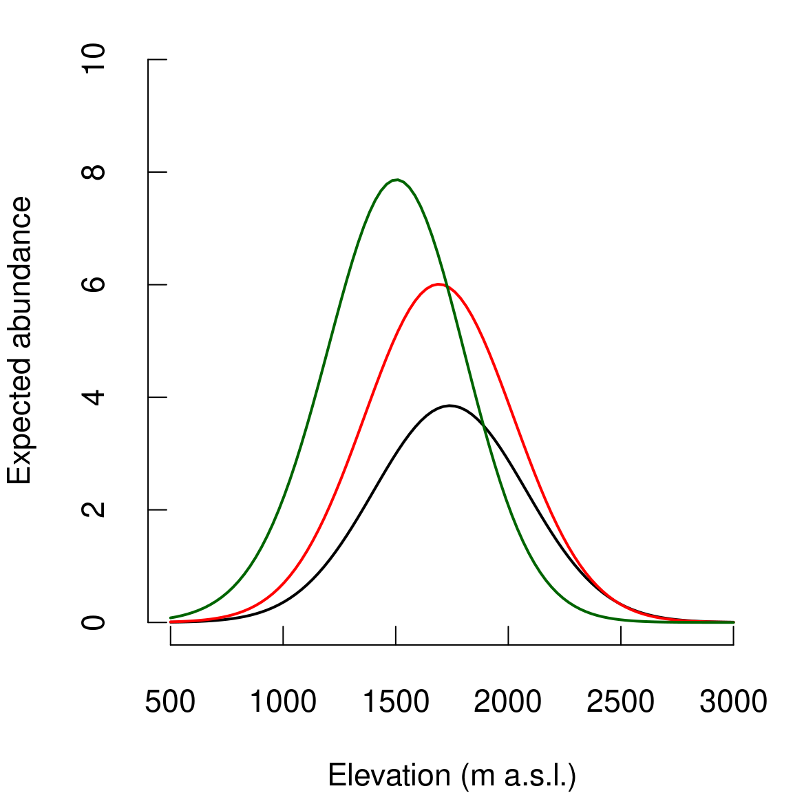
Figure 5.1: Relationship between abundance and altitude. Black: Poisson model, Red: N-mixture model, Green: N-mixture model with iCAR.
#lines(elev.seq,N.q1.Nmix.iCAR,lty=3,lwd=1,col="dark green")
#lines(elev.seq,N.q2.Nmix.iCAR,lty=3,lwd=1,col="dark green")
# Detection probability - Julian date
par(mar=c(4,4,1,1),cex=1.4,tcl=+0.5)
plot(juldate.seq,delta.est.Nmix,type="l",
     xlim=c(100,200),
     ylim=c(0,1),
     lwd=2,
     col="red",
     xlab="Julian date",
     ylab="Detection probability",
     axes=FALSE)
lines(juldate.seq,delta.q1.Nmix,lty=3,lwd=1,col="red")
lines(juldate.seq,delta.q2.Nmix,lty=3,lwd=1,col="red")
axis(1,at=seq(100,200,by=20),labels=seq(100,200,by=20))
axis(2,at=seq(0,1,by=0.2),labels=seq(0,1,by=0.2))
# Nmix.iCAR
lines(juldate.seq,delta.est.Nmix.iCAR,lwd=2,col="dark green")
lines(juldate.seq,delta.q1.Nmix.iCAR,lty=3,lwd=1,col="dark green")
lines(juldate.seq,delta.q2.Nmix.iCAR,lty=3,lwd=1,col="dark green")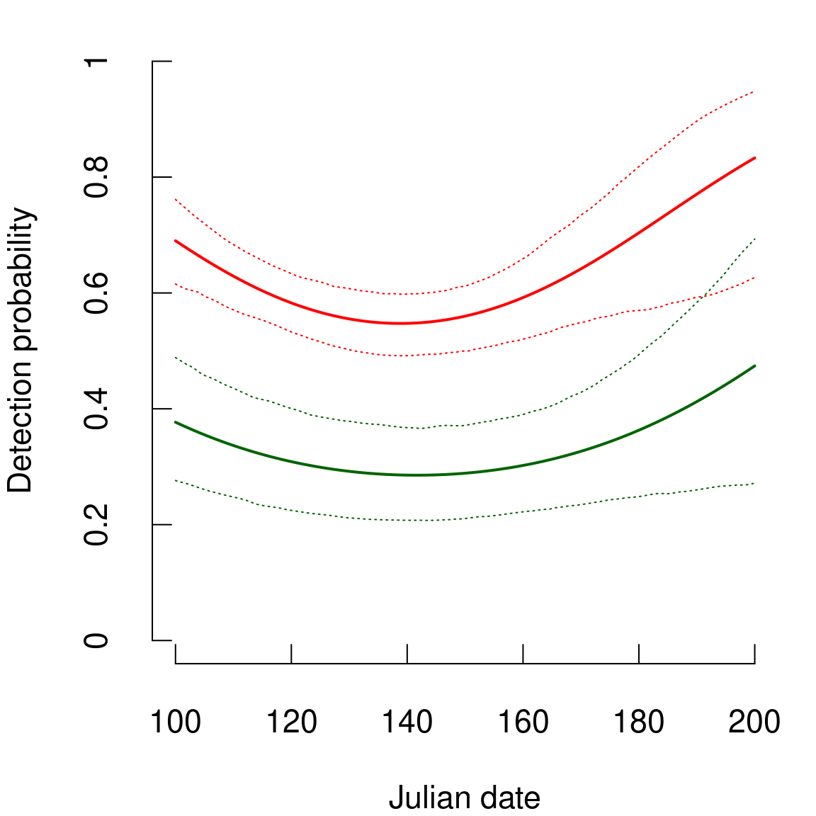
Figure 5.2: Relationship between detection probability and observation date. Red: N-mixture model, Green: N-mixture model with iCAR.