Country data

1 Introduction

This notebook presents the functions of the forestatrisk Python package that can be used to collect the spatial data needed for modeling and forecasting deforestation in a given country.

Data are retrieved from global (or pantropical) datasets freely available on the internet. Of course, the user can add any additional variables to the analyses manually. To do so, the user must add GeoTIFF raster files with extension .tif in the data folder of the working directory.

1.1 Importing Python modules

We import the Python modules needed for collecting the data.

# Imports
import os

from dotenv import load_dotenv
import ee
import pandas as pd
from tabulate import tabulate

from pywdpa import get_token
import forestatrisk as far

We create some directories to hold the data and the ouputs with the function far.make_dir().

far.make_dir("data_raw")
far.make_dir("data")
far.make_dir("output")

We increase the cache for GDAL to increase computational speed.

# GDAL
os.environ["GDAL_CACHEMAX"] = "1024"

1.2 Set credentials

We need to configure and set credentials for:

• Google Earth Engine (GEE) API

• RClone to access Google Drive

• WDPA API

You will need a Google account for using the GEE API and accessing Google Drive.

1.2.1 Access to Google Earth Engine API

Google Earth Engine is used to compute the past forest cover change from Vancutsem et al. 2021 or Hansen et al. 2013. To get credentials for using the Google Earth Engine API, follow these instructions. While authentication with ee.Authenticate() should be necessary only once, you have to execute the command ee.Initialize() at each session.

# Uncomment to authenticate for the first time.
# ee.Authenticate()
ee.Initialize(project="forestatrisk")

Under Linux and Mac, credentials are stored in $HOME/.config/earthengine/credentials.

cat $HOME/.config/earthengine/credentials

1.2.2 Access to Google Drive with RClone

RClone is used to download the forest cover change raster locally from Google Drive. To install RClone, follow these instructions. To configure the access to your Google Drive, follow these instructions.

1.2.3 Access to WDPA API

We will be using the pywda Python package to collect the data on protected areas from the World Database on Protected Areas (WDPA) at https://www.protectedplanet.net. To access the Protected Planet API, you must first obtain a Personal API Token by filling in the form available at https://api.protectedplanet.net/request. Then you need to set an environment variable (we recommend using the name WDPA_KEY) using either the command os.environ["WDPA_KEY"]="your_token" or python-dotenv.

The validity of your token can be checked with the function pywdpa.get_token().

# WDPA API
load_dotenv(".env")
get_token()

If your token is valid, the function will return its value. Otherwise it will print an error message.

2 Data

2.1 Compute forest cover change

We specify the iso3 code of the country we want the data for, for example Martinique.

iso3 = "MTQ"

We compute the past forest cover change from Vancutsem et al. 2021 using Google Earth Engine. The argument gdrive_remote_rclone of the function far.data.country_forest_run() specifies the name of the Google Drive remote for rclone. The argument gdrive_folder specifies the name of the Google Drive folder to use. In this case, folder GEE/GEE-forestatrisk-notebooks should exist in Google Drive.

# Compute gee forest data
far.data.country_forest_run(
    iso3, proj="EPSG:4326",
    output_dir="data_raw",
    keep_dir=True,
    fcc_source="jrc", perc=50,
    gdrive_remote_rclone="gdrive_gv",
    gdrive_folder="GEE/GEE-forestatrisk-notebooks")

2.2 Download raw data

# Download data
far.data.country_download(
    iso3,
    gdrive_remote_rclone="gdrive_gv",
    gdrive_folder="GEE/GEE-forestatrisk-notebooks",
    output_dir="data_raw")

Downloading data for country MTQ
SRTM not existing for tile: 25_09
Data for MTQ have been downloaded

2.3 Compute explanatory variables

We first set the projection in which we want the data to be, for example EPSG:5490.

# Projection
proj = "EPSG:5490"

We compute the explanatory variables from the raw data.

# Compute variables
far.data.country_compute(
    iso3,
    temp_dir="data_raw",
    output_dir="data",
    proj=proj,
    data_country=True,
    data_forest=True,
    keep_temp_dir=True)

2.4 Files

The data folder includes:

• Forest cover change data for the period 2010-2020 as a GeoTiff raster file (data/fcc23.tif).

• Spatial explanatory variables as GeoTiff raster files (.tif extension, eg. data/dist_edge.tif for distance to forest edge).

• Additional folders: forest, forecast, and emissions, with forest cover change for different periods of time, explanatory variables at different dates used for projections in the future, and forest carbon data for computing carbon emissions.

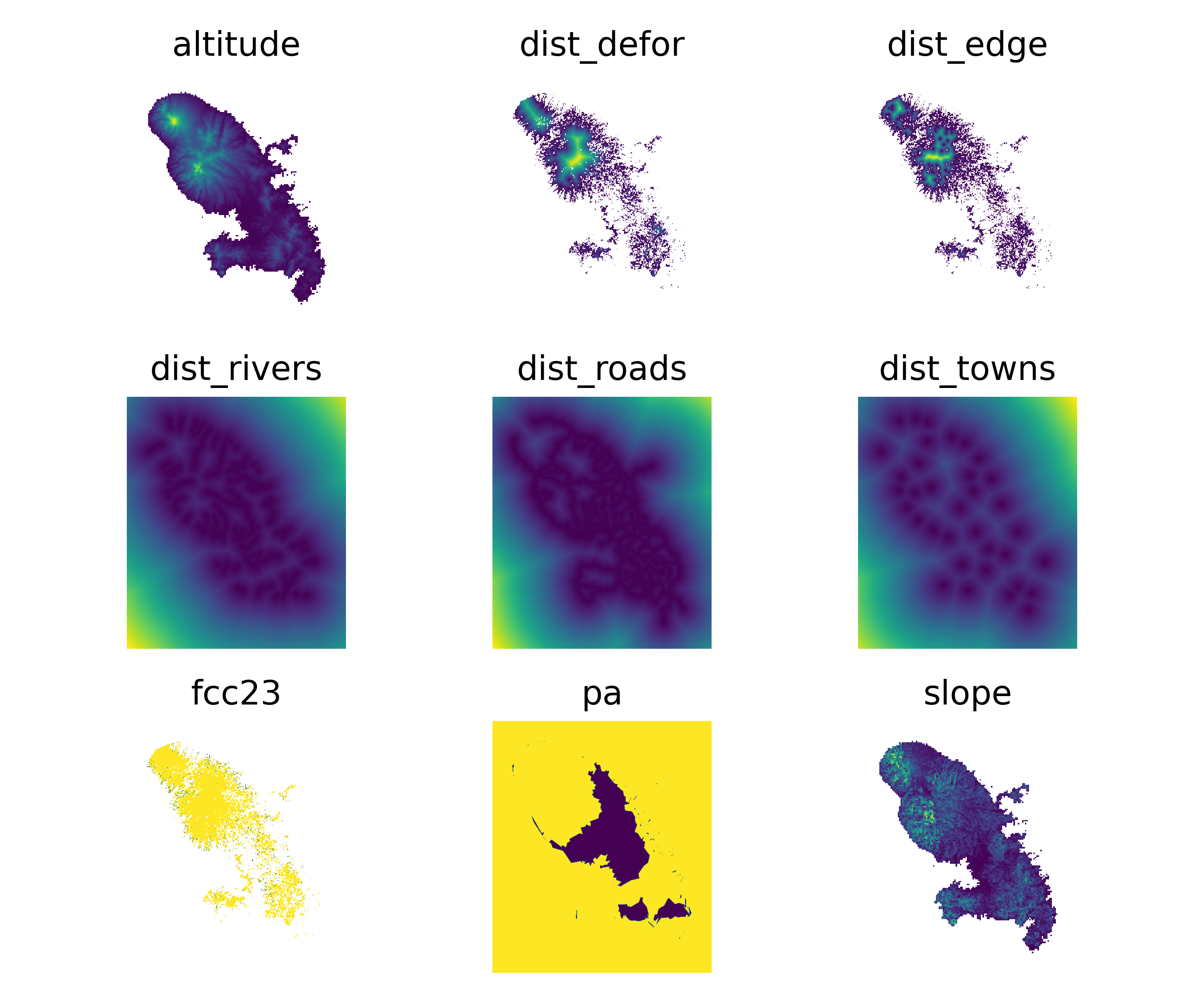
Variable characteristics are summarized in the following table:

Product	Source	Variable	Unit	Resolution (m)
Forest maps (2000-2010-2020)	Vancutsem et al. 2021	distance to forest edge	m	30
		distance to past deforestation	m	30
Digital Elevation Model	SRTM v4.1 CSI-CGIAR	altitude	m	90
		slope	degree	90
Highways	OSM-Geofabrik	distance to roads	m	150
Places		distance to towns	m	150
Waterways		distance to river	m	150
Protected areas	WDPA	protected area presence	–	30

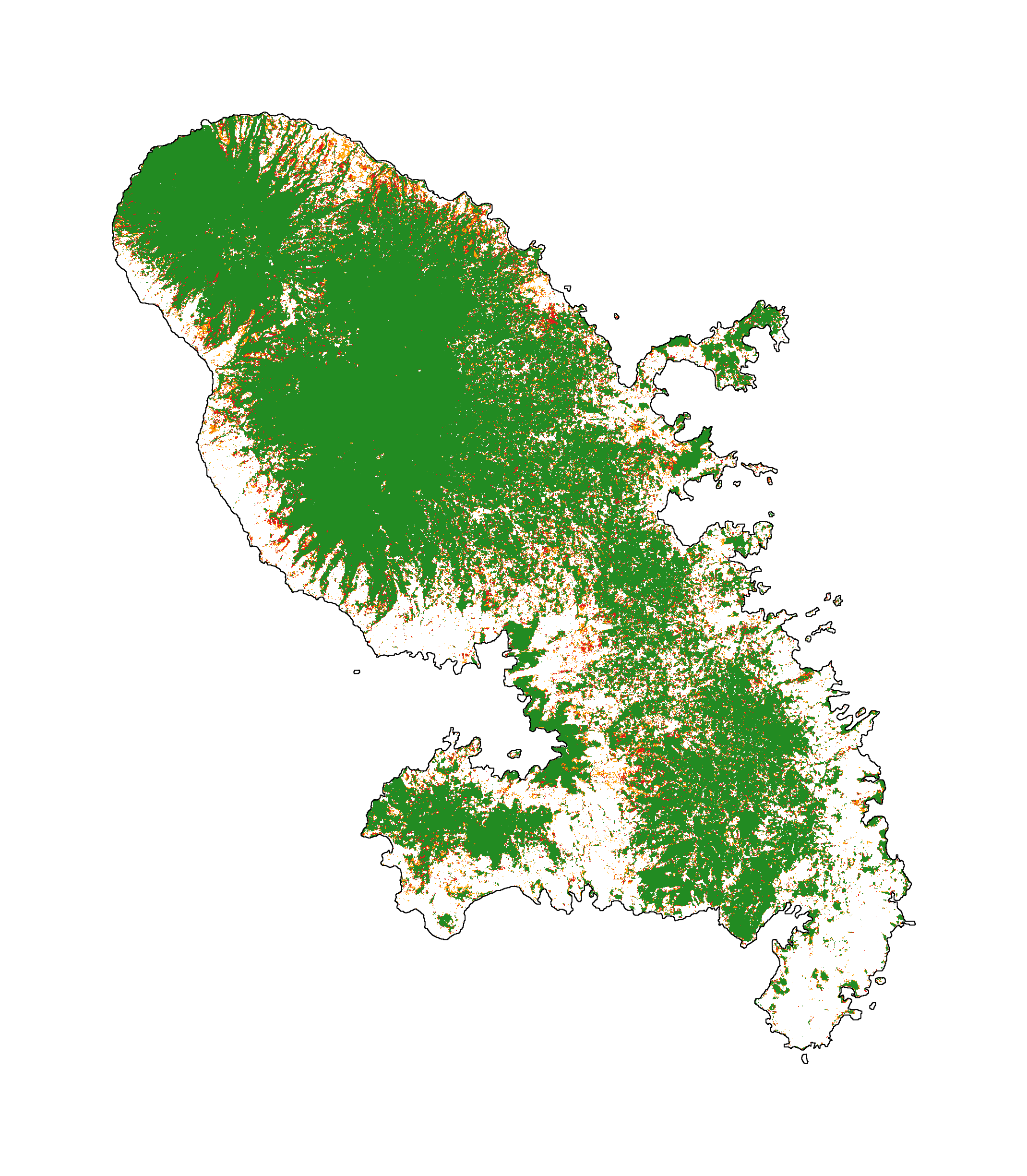
2.5 Plots

We can plot the past deforestation for the period 2000–2010–2020:

# Plot forest
ofile = "output/nb_ctrydata_fcc123.png"
fig_fcc123 = far.plot.fcc123(
    input_fcc_raster="data/forest/fcc123.tif",
    maxpixels=1e8,
    output_file=ofile,
    borders="data/ctry_PROJ.shp",
    linewidth=0.3,
    figsize=(6, 5), dpi=500)
ofile

We can also plot the explicative variables:

# Plot explicative variables
ofile_pdf = "output/nb_ctrydata_var.pdf"
ofile = "output/nb_ctrydata_var.png"
fig_var = far.plot.var(
    var_dir="data",
    output_file=ofile_pdf,
    figsize=(6, 5), dpi=500)
fig_var[0].savefig(ofile)
ofile