Initialisation
Load shapefile of Grande Terre borders. Our study is only on Grande Terre because there isn’t inventory on others island of New Caledonia.
We also need environmental and climatic variables for compute JSDM
model. You can use gecevar to extract easily all data.
Those file are crop to keep only data of Grande Terre.
Create moist forest mask
We need to keep only moist forest that isn’t mangrove. To do this we remove all forest with an altitude < 10m. For moist forest, we use FAO definition ( MAP >=1500 mm, <5 months where precipitations < 100 mm).
elevation <- rast(here("output", "dataNC.tif"))["elevation"]
forest_per <- rast(here("output", "dataNC.tif"))["forest"]
forest <- create_sf_forest(EPSG = EPSG, altitude_min = 10, percentage_min = 50, elevation = elevation, forest = forest_per)
monthly_precipitation <- rast(here("output", "current_chelsaNC.tif"))[[paste0("pr", 1:12)]]

moist_forest_sf <- create_sf_moist_forest(EPSG = EPSG,
                                          forest = forest,
                                          monthly_precipitation = monthly_precipitation)
write_sf(moist_forest_sf, here("output", "moist_forest.shp"))
Create explanorities variables for JSDM algorithme
Create a Tiff file with only needed variables. You can select variables you want and power of each variables.
data_NC <- read_stars(here("output", "dataNC.tif")) # gecevar merge with peridotites
var_jSDM <- extract_var_JSDM(stars_object = data_NC,
                             variables_names = c("peridotites", "bio1", "bio4", "bio12", "bio15", "cwd"),
                             power_variable = c(1, rep(2,5)),
                             scale = c(FALSE, rep(TRUE, 5)))
write_stars(merge(var_jSDM), here("output", "var_jSDM.tif"), options = c("COMPRESS=LZW","PREDICTOR=2"))

coord_site <- read.csv2(here("data_raw", "NCpippn", "coord_site.csv"), sep = ",")
coord_site[, "AREA"] <- 0
NC_PIPPN <- read.csv2(here("data_raw", "NCpippn", "data_clear.csv"), sep = ",")

for (site in 1:dim(coord_site)[1]) {
  coord_site$AREA[site] <- as.numeric(NC_PIPPN$AREA[coord_site$plot_name[site] == NC_PIPPN$plot_name][1])
}
var_site <- data_JSDM(EPSG = EPSG,
                      latlon_site = coord_site[, 2:3],
                      area_site = coord_site$AREA,
                      path_tiff = here("output", "var_jSDM.tif"),
                      log_area_site = TRUE)
jSDM binomial probit
Compute jSDM binomial probit method with jSDM package.
Only mean options of jSDM_binomial_probit are available.
Display some plot to check if jSDM_binomial_probit model
run well. All plots, are about inventories sites.
PA <- read.csv2(here("data_raw", "NCpippn", "Presence_Absence.csv"), sep = ",")
PA$X <- NULL
jSDM_bin_pro <- JSDM_bino_pro(PA = PA,
                              site_data = var_site,
                              n_latent = 2,
                              V_beta = c(rep(1, 12), 0.001),
                              mu_beta = c(rep(0, 12), 0.25),
                              nb_species_plot = 2,
                              display = TRUE,
                              save_plot = TRUE)

save(jSDM_bin_pro, file = here("jSDM_bin_pro.RData"))
load(here("jSDM_bin_pro.RData"))
plot_pres_est_one_species(jSDM_binom_pro = jSDM_bin_pro,
                          coord_site = coord_site,
                          country_name = "New Caledonia",
                          display_plot = TRUE,
                          save_plot = TRUE)

plot_species_richness(jSDM_binom_pro = jSDM_bin_pro,
                      coord_site = coord_site,
                      country_name = "New Caledonia",
                      display_plot = TRUE,
                      save_plot = TRUE)
kNN interpolation
Compute a k-Nearest Neighbors interpolation on site-effect alpha and latent variables. So we can get probabilities of presence for each species on each pixel of forest.
This function takes around 25min to run.
knn_interpolation_jSDM(jSDM_binom_pro = jSDM_bin_pro, k = 5, coord_site = coord_site, sf_forest = moist_forest_sf)Probabilities on forest area and plots
Compute from kNN interpolation a map with probability of presence for each species on each pixel of forest in Grande Terre.
In this case we remove alpha for compute probabilities of presence to avoid high species richness values. This process doesn’t change the order of probabilities in pixel.
Plot of species richness on New Caledonia forest.
alpha <- read_stars(here("output", "alpha_knn.tif"))
W1 <- read_stars(here("output", "lv_1_knn.tif"))
W2 <- read_stars(here("output", "lv_2_knn.tif"))
W <- c(W1, W2, along = "band")
var_jSDM <- st_crop(var_jSDM, forest)

prob_est_species_forest(alpha_stars = alpha,
                        latent_var_stars = W,
                        jSDM_binom_pro = jSDM_bin_pro,
                        data_stars = var_jSDM)

plot_prob_pres_interp(theta_stars = read_stars(here("output", "theta", "KNN_theta_01.tif")),
                      country_sf = GT,
                      display_plot = TRUE,
                      save_plot = TRUE)

species_richness_terra <- plot_species_richness_interpolated(list_theta_path = list.files(here("output", "theta"), full.names = TRUE),
                                                             country_sf = GT,
                                                             display_plot = TRUE,
                                                             save_plot = TRUE,
                                                             save_tif = TRUE)
Dimension reduction
At this point dimensions are \(nb\ of\ species \times nb\ of\ pixel\). We need to reduce dimensions to clustering pixel in comunities. Decrease dimensions using PCA or tSNE method then determine number of communities with dendrogram compute with HCA.
Big drop-off in dendrogram are “good” numbers of groups. If dendrogram doesn’t have drop-off with one reduction dimension method, use the other method. There is few way to shape the number of groups, HCA is one of them. HCA is also a clustering method but for now we areusing it only for number of groups.
coord_PCA_or_tSNE <- PCA_or_tSNE_on_pro_pres_est(tSNE = TRUE,
                                                 PCA = FALSE,
                                                 list_theta_path = list.files(here("output", "theta"), full.names = TRUE),
                                                 display_plot = TRUE,
                                                 save_plot = TRUE)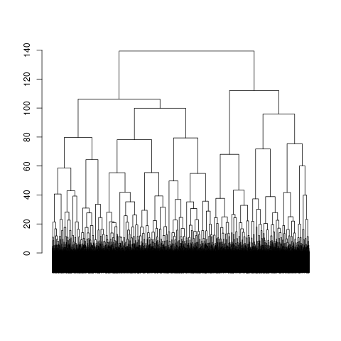
Clustering
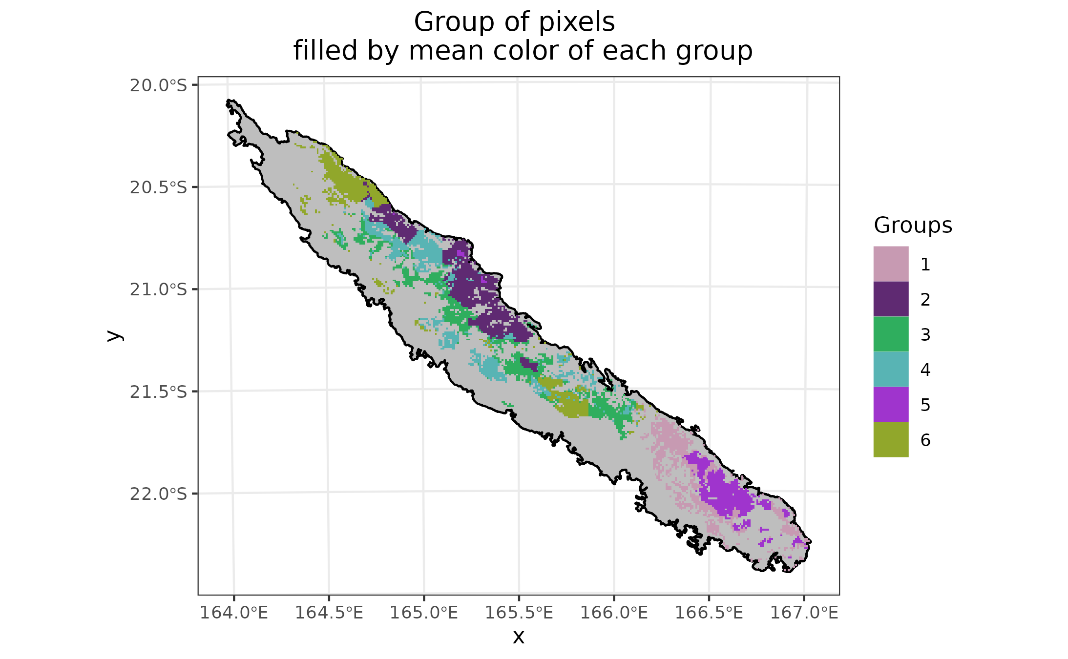
Pixel’s clustering is computing with a method among HCA, kmeans or Expectation-Maximisation (EM). In this case, we choose kmeans because we wanted to have groups strong to perturbations. But this criteria can be modify for the purpose you are following. With our data, kmeans is the better method by far. Create outputs to visualize clustering in the first three dimensions of PCA or tSNE.
KM_groups <- plot_HCA_EM_Kmeans(method = "KM",
                                pixel_df = coord_PCA_or_tSNE,
                                nb_group = 6,
                                display_plot_3d = TRUE,
                                display_plot_2d = TRUE,
                                save_plot_2d = TRUE)
Plot with colors and groups
Plot New Caledonia map with values in of the first three axis of PCA or tSNE method for each pixel. To see impacts of each axis on pixels. Those plots have different colors (Red, Green, Blue) for each axis of PCA or tSNE. To see diversity \(\beta\), display three plots in one. This plot in a RGB plot, similar colors are pixels with similar trees communities. Plot groups on New Caledonia map with mean color of each group.
pixels_group <- split(read_stars(here("output", "theta", "KNN_theta_01.tif")))[1,,]
pixels_group[[1]][!is.na(pixels_group[[1]])] <- KM_groups
names(pixels_group) <- "groups"

plot_RGB_group_by_color(stars_pixels_group = pixels_group,
                        coord_pixel = coord_PCA_or_tSNE,
                        country_sf = GT,
                        display_plot = TRUE,
                        save_plot = TRUE)

max_min_df <- max_min_species_group(list_theta_path = list.files(here("output", "theta"), full.names = TRUE),
                                    stars_pixels_group = pixels_group,
                                    nb_top_species = 20,
                                    save_csv = TRUE)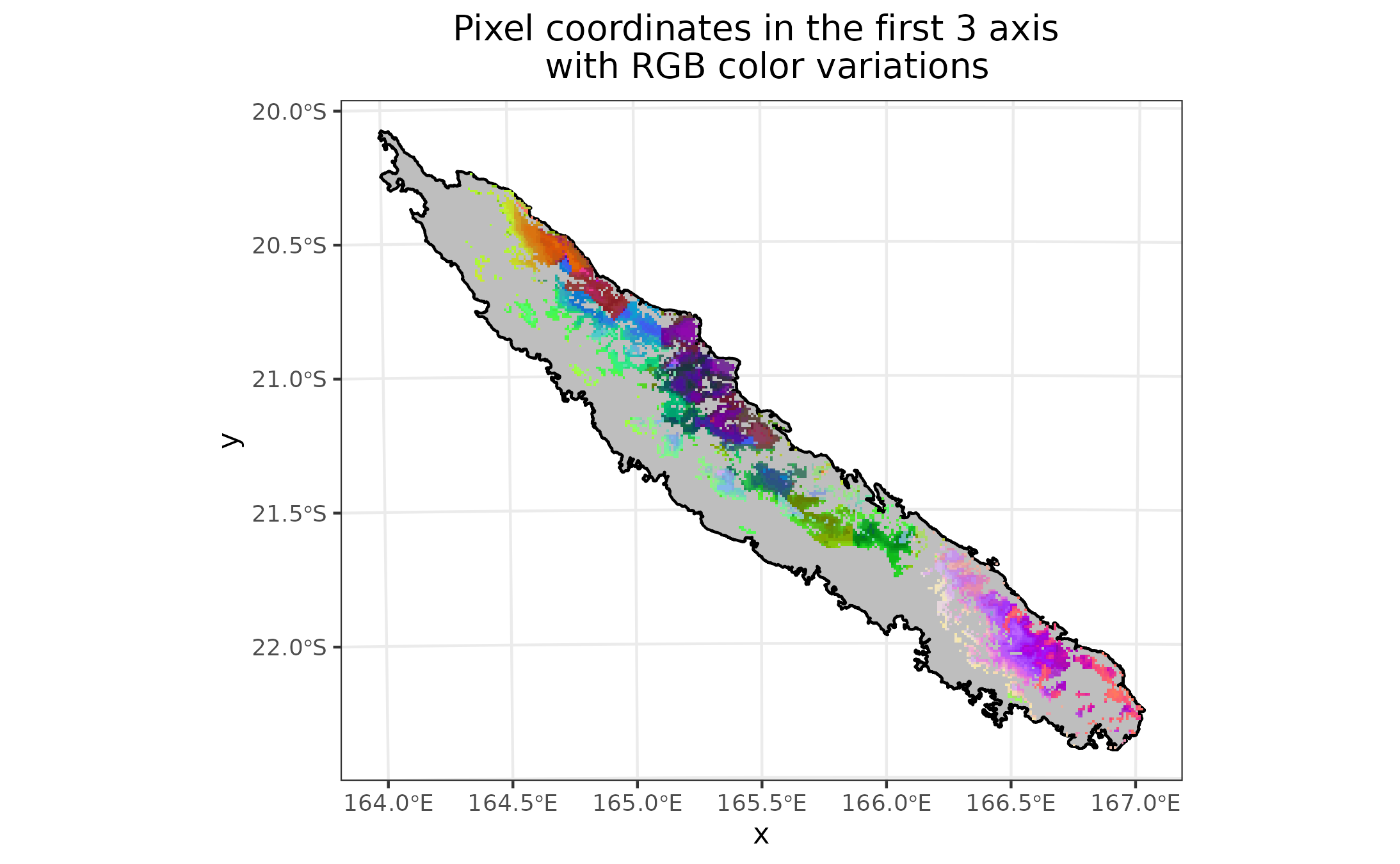
Sensibility & Specificity
Sensibility and specificity are calculated on inventories sites without cross validation. True Skills Statistic (TSS) is great above 0.7
sens <- sensitivity(PA = PA, jSDM_binom_pro = jSDM_bin_pro)
spe <- specificity(PA = PA, jSDM_binom_pro = jSDM_bin_pro)
TSS <- sens + spe -1
TSS